
Abstract
Operations research (OR) is a branch of applied mathematics dedicated to analytical decision-making, and has close ties with optimization, statistics, and mathematical modeling. As a discipline, it is often housed in schools of engineering or business, and undergraduate students of mathematics may have little exposure to the field. However, for students interested in practical applications of mathematics, operations research contains a wonderful abundance of problems. In this brief introduction, we discuss two classes of optimization problems of interest to operations research, linear programs (LP) and their generalization, convex programs. Both theory and applications are outlined. We also mention project ideas that could be pursued by undergraduates.
Access provided by CONRICYT-eBooks. Download chapter PDF
Keywords
- Operations research
- Optimization
- Decision-making
- Applied mathematics
- Linear programming
- Convex programming
Differential calculus, Linear algebra.
1 Introduction
The Institute for Operations Research and the Management Sciences (INFORMS) defines operations research (OR) as “a discipline that deals with the application of advanced analytical methods to help make better decisions.” It uses tools and techniques from mathematics, including modeling, statistics, data analysis, and optimization, to find a maximum (profit, yield) or minimum (cost, risk) solution to a problem, typically in the presence of one or more system constraints. OR as a discipline began during World War II with the study of military planning and resource allocation problems, and as such, has had an applied focus from its inception. Today, principles of OR are widely used in business practice, and OR is a well-established research field.
OR’s application-driven focus lends itself excellently to a variety of practical research problems of interest to industry, from scheduling to allocation to management. At the same time, OR stands on rigorous mathematical footing, and students with a more theoretical bent will have no shortage of problems involving structural properties, uniqueness of solutions, and algorithms.
There are many classes of optimization problems that are of interest in OR applications. A non-exhaustive list follows:
-
Linear programming: The problem of optimizing a linear objective function subject to linear equality and inequality constraints. The subject gained popularity due to the development of the Simplex method, one of the first reliable and efficient optimization algorithms. (It should be noted that the word “program,” in the OR context, is used to mean an optimization problem, and its use predates that of computer programs.)
-
Convex programming: A generalization of linear programming, convex programming is the problem of optimizing a convex objective function subject to convex constraints. Many practical optimization problems can be formulated (or re-formulated) as convex problems. Again, efficient algorithms for the solution of convex problems have been developed, especially for problems of certain standard forms; thus, formulation of a problem as convex often leads to computational tractability.
-
Integer programming: The problem of optimizing a linear objective function subject to linear equality and inequality constraints, in which some or all variables are constrained to be integer-valued. Integer programs are non-convex and are generally much more difficult to solve than linear programs.
-
Stochastic programming: The problem of optimizing a system in which some or all constraints or parameters depend on random variables.
-
Dynamic programming: A technique for solving an optimization problem by separating it into a collection of simpler sub-problems. Among other applications, they are useful for sequential decision-making, where the problem of reaching some optimal state in the future is broken down into a series of finite or countable individual problems at each time step.
-
Combinatorial/network optimization: The problem of determining a discrete optimal object from a finite set of objects on a graph, a set of vertices with arcs connecting pairs of vertices. The famous Traveling Salesman problem of finding a minimum-distance route connecting a known set of points is one such example.
In applications, oftentimes combinations of these problem classes are used. However, in this short introduction, we focus on just the first two classes of problems: linear programs and convex programs.
In these problems, there are two different sorts of quantities of interest: parameters and decision variables. Parameters are typically known and are treated as constants for the purposes of solving the problem. Decision variables are the values that we seek. For example, in determining a shortest-distance route between two points on a map, the parameters would be the (fixed) distances of each road segment, which are known; the decision variable would be the sequence of segments that we decide to travel on. After the problem has been solved and we have a value for the decision variables, we are often interested in how our solution depends on the parameter values. In the example, how would our route change if any particular segment on the map had been shorter, or longer, or removed altogether? This procedure is called sensitivity analysis.
In this paper, we begin with linear programming, then move to the more general convex programming, explaining the theory, providing examples, and describing possible research ideas for both. We conclude with pointers to further reading as well as software tools for solving these problems.
2 Linear Programming
A linear program (LP) is a technique for optimization (minimization/maximization) of a linear objective function subject to linear equality and inequality constraints. Software packages exist for efficient solution of LPs, even in high dimensions with many variables and constraints. Thus, formulating a problem as a LP is often computationally advantageous. LPs have been used in many applications, including shift scheduling, network design, and manufacturing. We begin this section with an example, the diet problem. We then discuss a general formulation of LPs, as well as algorithms for their solution. Finally, we end with a discussion of duality.
2.1 Diet Problem
Let us illustrate the basic idea through an example. We wish to construct a daily diet with the minimum possible cost. The diet is selected from certain candidate foods and must satisfy certain nutritional requirements. To begin, we consider only two candidate foods: milk and bread; and four nutritional requirements: protein, carbs, vitamins, and sugar. The parameters are given in the following chart.
Let m be the number of units of milk to consume, and b the number of units of bread; these are our decision variables. We seek m and b to minimize the total cost:
subject to the constraints:
Here, the first, second, and third constraints correspond to the minimum requirements for protein, carbs, and vitamins, respectively. The fourth constraint corresponds to the maximum requirement for sugar. The fifth and sixth constraints are non-negativity constraints that ensure a physically meaningful result.
Since we have only two variables, we can easily plot the constraints on a pair of axes. The region where all constraints are satisfied is known as the feasible region or feasible set, and points in the feasible region are called feasible points. On Figure 1, the feasible region is labeled R. On the same plot, we show dotted lines of constant cost: where 0. 3m + 0. 2b is a constant. By moving in a direction of decreasing cost, we can visually see that the lowest-cost point within the feasible region occurs at point P, at (m, b) = (0. 5, 1. 5), which is also a vertex of R. The cost at point P is the value of the objective function there: 0. 3(0. 5) + 0. 2(1. 5) = 0. 45.

Constraints (solid lines), feasible region (R), and lines of constant cost (dotted lines) for the diet problem.
Upon viewing Figure 1, we make several observations. First, the feasible region will always be a convex polygon. (It may be bounded or unbounded.) In 2D, we can think of a convex polygon as one in which all interior angles are ≤ 180∘; a more general definition of convexity is discussed in section 3.1. In higher dimensions, this generalizes to a convex polytope.
Second, in this problem, the unique solution was a vertex. This will become important later when we discuss solution algorithms.
2.2 Standard Forms
We now consider a general minimization LP. To avoid trivialities, assume that the feasible region R is non-empty and that the objective function is bounded below within R. Then there exists an optimal solution which is a vertex of the feasible region. (A proof of this statement is given in section 2.6 of Bertsimas and Tsitsiklis [2]). If there are multiple, non-unique solutions, they occur at an entire edge (or face, in higher dimensions,) of R. Going back to the diet problem for a moment, this would have happened happen if the lines of constant cost were parallel with one of the three minimum requirements of Figure 1. Even in this case, there still exists a solution at some vertex (in 2 dimensions, the vertices on either end of a polygon edge). Since in a typical decision-making framework we only need one solution to implement, the issue of uniqueness is less important, and we may restrict our search for the solution to only vertices of the feasible region. This is a key motivation for the Simplex method, which will be discussed shortly.
Let \(x \in \mathbb{R}^{n}\) be a vector containing the n decision variables and \(c \in \mathbb{R}^{n}\) be a vector containing the parameters representing coefficients of each corresponding variable in the objective function. Assume the ith inequality constraint out of m total is of the form ∑ j = 1 n a ij x j ≥ b i ; then, all such constraints can be succinctly written in matrix-vector notation as Ax ≥ b, where \(A \in \mathbb{R}^{m\times n}\) is a matrix containing the coefficients of the constraint functions (including non-negativity constraints), \(b \in \mathbb{R}^{m}\) is a vector of the constraint right-hand side values, and “ ≥ ” is meant in the component-wise sense. (We will shortly show that this assumption is not restrictive.) If this is the case, then one general form of an LP is:
We have denoted transpose by ′; thus, c′x = ∑ i = 1 n c i x i . Other constraints can be put into the form ∑ j = 1 n a ij x j ≥ b i as well: “ ≤ ” inequality constraints of the form a ij x j ≤ b i can be changed to greater-than through multiplication by − 1, and “=” constraints of the form a ij x j = b i can be written as the pair of inequality constraints a ij x j ≥ b i and − a ij x j ≥ −b i . Finally, any linear maximization problem maxc′x is equivalent to min − c′x.
The feasible region \(R \subseteq \mathbb{R}^{n}\) is the set of points satisfying the constraints:
Geometrically when R exists it is a convex polytope.
While the general form (3) is geometrically intuitive, from an algorithmic standpoint, it is often more convenient to write the constraints in a slightly different way. Namely, we can equivalently define R of (4) as
for a different A, x, and b. Namely, equality constraints of the form a ij x j = b i are left alone, while inequality constraints are converted to equality constraints via the introduction of so-called “slack” or “surplus” variables. We proceed by example. Consider the “ ≤ ” constraint:
We introduce a new nonnegative variable x 4, called the slack variable. Equation (6) can then be written equivalently as a pair of equality and non-negativity constraints:
A “ ≥ ” constraint can be handled in a similar way by introducing a so-called surplus variable. The final conversion is to eliminate free variables, that is, variables that are not restricted to be non-negative or non-positive. If x 6 is a free variable, we eliminate it and introduce two new non-negative variables x 7, x 8. The free variable x 6 can then be replaced with
The LP with constraints written in the aforementioned form:
is referred to as a “standard-form” LP.
Research Project 1.
Develop a more realistic diet problem using nutritional data and formulate it as an LP. For example, Bosch compared several fast food chains to determine which, if any, offered a combination of entrees could meet federal dietary guidelines at lowest cost [3]. Bosch’s formulation was an integer program, where one or more variables is restricted to be integer-valued. However, by relaxing this assumption, an analogous LP can be developed.
Research Project 2.
Scheduling problems are a classic area of interest in OR. Develop a minimum-cost schedule for a company in which employees work on various tasks by formulating the problem as a LP. Constraints could include, but are not limited to, working hours for every individual employee; total working hours spent on each task; and penalizing shift changes to avoid frequent off-and-on times for each employee.
2.3 Solution of LPs
Many algorithms for solving LPs operate by first finding a feasible point and then iteratively moving in a direction of improving objective function value. Because the objective function is linear, any local optimum is also a global optimum; thus, a greedy algorithm will find an optimum eventually. Once a feasible solution has been found that moving in any direction would result in a worse objective function value, the algorithm terminates. Algorithms for LPs thus often have an easily understandable geometric interpretation. The main difficulty in solving LPs is that most problems of interest lie in a high-dimensional space, oftentimes with thousands (or more) of variables and constraints.
In optimization, algorithmic computational complexity is often described in terms of strongly polynomial, weakly polynomial, or non-polynomial time. We assume basic arithmetic operations of addition, subtraction, multiplication, division, and comparison take one time step to perform. The number of operations in a weakly polynomial time algorithm is bounded by a polynomial in the number of constraints and variables. For an algorithm to be strongly polynomial time, additionally the memory used by the algorithm must be bounded by a polynomial in the number of constraints and variables. Certain algorithms including interior-point methods are weakly polynomial; however, no strongly polynomial method has yet been found for LPs. In fact, the existence of such an algorithm was listed on Stephen Smale’s 18 open problems of mathematics for the 21st century [13]. Nevertheless, there is a fortunate disconnect between theoretical and practical notions of run time, in that algorithms exist for solving in LPs that are highly efficient for many practical problems of interest, despite the fact that they are not strongly (or in many cases, even weakly) polynomial in theory.
The first efficient algorithm for solving LPs was the Simplex method, developed by George Dantzig in the 1940s. The Simplex method has an intuitive geometrical interpretation and was widely used for several decades; even today, it lies at the heart of many LP solvers.
2.3.1 The Simplex Method
Without loss of generality, we consider a minimization problem. The Simplex method begins with a subroutine to find a vertex of the feasible region, if one exists. It then chooses the edge of the polytope with the fastest decrease (steepest descent) in objective function. It then moves the solution along that edge until hitting a vertex; then repeats. There are certain caveats to take into consideration at so-called degenerate points, where several constraints coincide at the same point, and when a tie for the steepest descent direction occurs, but the essential geometry is shown in Figure 2.

A toy problem in 3 variables: the feasible region is a 3-dimensional convex polyhedron. The Simplex method, depicted with a red arrow, follows edges from vertex to vertex in a direction of improving (decreasing, for a minimization problem) objective function value.
The run time is, in theory, exponential in the number of variables. Indeed, a worst-case scenario for an n-variable problem was found by Klee and Minty where the Simplex method visits every vertex of a perturbed n-dimensional hypercube, of which there are 2n, before finding the optimal solution [8]. Nevertheless, the average behavior of the Simplex method on problems of interest seems to be significantly better. Of course, we have not provided a rigorous definition of “average behavior”; indeed, the problem of defining such a concept and using it to define the run time of Simplex method remains somewhat open [1, 12].
Research Project 3.
Define an appropriate notion of average-case behavior for the Simplex method. Computational experiments can be performed by generating random problems according to some probabilistic setup, and finding the run time of the Simplex method on each. Then, using regression, find the relationship between the mean and variance of the observed run times as a function of the problem size (number of variables + constraints).
2.3.2 Interior Point Methods
In contrast to the Simplex method, where the algorithm visits vertices of the feasible polytope by traveling along edges of the region, interior point methods travel through the interior of the feasible region. The basic idea in interior point methods is to choose a path that optimizes a combination of a reduction in objective value function and the distance from the edge of the feasible region. This is often done through the introduction of a barrier function: a function that is inversely proportional to the distance from the nearest edge of the polytope and thus carries low values in the center and approaches + ∞ on the edge itself. Let us introduce a scalar α ≥ 0 that indicates the relative importance of the barrier function as compared with the change in the objective value function c′x. By minimizing an appropriate sum of the objective function value and α times the barrier function, we find a path through the interior of the feasible region that depends on α. This path is counterintuitive, as the barrier function avoids the boundary of the feasible region, when it is known that all solutions lie on the boundary. However, by letting α → 0, we can then recover the optimum of the original objective function.
Interior point methods have been developed which are weakly polynomial-time in the number of variables. In practice they are often competitive with the Simplex method and similar edge-tracing algorithms, and for some sparse problems are significantly faster.
2.4 Transportation Problem
The following example illustrates another application that can be modeled as a LP. In order to produce a certain product, raw material must be transported from the mine to a plant where it is refined. Say a company has control over 2 mines in Colorado and Virginia, and 3 plants in Alabama, Minnesota, and New Mexico. We denote the mines C and V, and plants A, M, and N, respectively. Below is a table of the parameters representing estimated shipping costs between each plant and mine, in thousands of dollars per ton of material (Table 1).

For a certain week, the Colorado mine is expected to output 150 tons of ore, and the Virginia mine 130. To fulfill demand in the same week, the Alabama plant requires at least 88 tons of ore, the Minnesota plant 125 tons, and the New Mexico plant 55 tons.
Exercise 1.
-
(a)
Formulate the problem as a linear program. Denote x CA as the decision variable for the amount of ore shipped (in tons) from Colorado to Alabama, etc.
-
(b)
A colleague suggests that it would be easiest if the Colorado mine exclusively supplied New Mexico and Alabama, and the Virginia mine exclusively supplied Minnesota (only enough to meet demand.) Check that this option is feasible. Find the total shipping cost (in thousands of dollars) in this case.
-
(c)
Solve for all x values using an off-the-shelf linear program solver. What is the total shipping cost (in thousands of dollars) in this case? How much did we save as compared to part (b)?
Solution 1.
-
(a)
$$\displaystyle{\min \qquad 22x_{CA} + 18x_{CM} + 7x_{CN} + 14x_{V A} + 20x_{V M} + 24x_{V N}}$$$$\displaystyle{\begin{array}{lrl} \text{subject to}& x_{CA} + x_{CM} + x_{CN}& \leq 150 \\ & x_{V A} + x_{V M} + x_{V N}& \leq 130 \\ & x_{CA} + x_{V A}& \geq 88 \\ & x_{CM} + x_{V M}& \geq 125 \\ & x_{CN} + x_{V N}& \geq 55 \\ &x_{CA},x_{CM},x_{CN},x_{V A},x_{V M},x_{V N}& \geq 0\end{array} }$$
-
(b)
$$\displaystyle{x =\big [x_{CA},x_{CM},x_{CN},x_{V A},x_{V M},x_{V N}\big]' =\big [88,0,55,0,125,0\big]'}$$$$\displaystyle{c'x =\big [22,18,7,14,20,24\big]\big[88,0,55,0,125,0\big]' = 4831}$$
-
(c)
$$\displaystyle{x =\big [x_{CA},x_{CM},x_{CN},x_{V A},x_{V M},x_{V N}\big]' =\big [0,95,55,88,30,0\big]'}$$$$\displaystyle{c'x =\big [22,18,7,14,20,24\big]\big[0,95,55,88,30,0\big]' = 3927}$$
This solution represents a savings of 4831 − 3927 = 904 dollars.
Research Project 4.
Formulate the problem of delivering electricity to consumers as a LP. Electricity must be delivered to meet demand and can come from a variety of sources, such as coal, natural gas, wind, and solar. Investigate the effect of a carbon tax on the solution by penalizing electricity coming from nonrenewable resources. Consider how future growth in a certain geographic area will affect the solution.
2.5 Duality
In calculus, students are typically taught the Lagrange multiplier method for optimizing functions subject to equality constraints. The key idea there is to introduce a new scalar parameter for each equality constraint (the multiplier), and reformulate the hard constraints as soft constraints additively combined with the original objective function (and scaled by the appropriate multiplier)– this quantity is the Lagrangian L. The new problem is to optimize L with no constraints. Assuming differentiability of L, this can be solved by equating the partial derivatives of L with zero. For the proper choice of the multipliers, the presence or absence of each hard constraint does not affect the optimal value of the objective function; thus, the optimal solution to the original constrained problem and the new unconstrained problem are the same.
Duality theory is a generalization of the Lagrange multiplier method that also accounts for inequality constraints. We again associate a multiplier with each constraint and seek a set of values for the multipliers such that the specific value of the constraint does not affect the optimal objective function value. We consider the standard-form LP of (9), which we call the “primal” problem. Let x ∗ be an optimal value of x, and assume x ∗ exists. We relax the standard-form problem by changing the hard constraint Ax − b = 0 to a soft one with the introduction of a length-m vector of multipliers λ. We then have the problem:
Let g be the optimal value of this relaxed problem. Since g depends on λ, let us consider it to be a function: g(λ). The relaxed problem is broader than the original problem in that if Ax = b, we recover the original problem, but there are also feasible points in which Ax ≠ b. In other words, the feasible region of the relaxed problem R′ contains the feasible region of the original problem R: R ⊆ R′. For this reason, the minimum value of the objective function in R′ must be no larger than the minimum value in R.
Here, the inequality arises because x ∗ is a member of the set x ≥ 0 and thus is a feasible solution to the primal problem, and the final equality is due to the fact that x ∗ satisfies Ax ∗ = b because it again is a feasible solution to the primal problem. Thus, g(λ) is a lower bound for the optimal cost c′x ∗.
Now consider the unconstrained problem:
This problem gives us the tightest possible lower bound for the optimal cost c′x ∗. This problem is known as the dual problem. Strong duality proves that the optimal cost of the dual problem is equal to the optimal cost c′x ∗ of the primal problem (see Theorem 4.4 of Bertsimas and Tsitsiklis [2]). Continuing a bit further, we have
Noting that the quantity (c′ −λ′A)x can be made arbitrarily small unless c′ −λ′A ≥ 0, we restrict our search in the dual problem to c′ −λ′A ≥ 0. The dual problem then becomes, in its final form:
One important feature of duality is that the dual of the dual of a primal problem is itself (see Theorem 4.1 of Bertsimas and Tsitsiklis [2]). Because of the correspondence of the solutions of the primal and dual problems, solvers can make use of both the primal and dual problems in searching for a solution. For example, a dual Simplex method can be developed that pivots on the vertices of the dual problem’s feasible region.
3 Convex Programming
In this section we investigate the problem of minimizing convex problems, which are defined as minimizing a convex function subject to convex constraints. Formally, the problem is:
where \(x \in \mathbb{R}^{n}\) are the variables, \(f_{0}: \mathbb{R}^{n} \rightarrow \mathbb{R}\) is the objective function, and \(f_{i}: \mathbb{R}^{n} \rightarrow \mathbb{R},\quad i = 1,\ldots,m\) are the constraint functions, and the objective and constraint functions are convex. We define convexity in the sections to follow.
In general, convex optimization problems do not have analytical solutions, but there do exist efficient algorithms for their solution. Convex programs are more general than linear programs and a large number of problems can be formulated as convex problems, though there are some tricks and such a formulation can often feel more of an art than a science.
In this section, we begin by defining convex sets and functions. We then give several well-known examples of classes of problems that are convex, before concluding with a mention of some software packages for solving convex problems.
3.1 Convex Sets
Whereas linear programs have feasible regions that are convex polytopes, convex programs have feasible regions that are general convex sets. A set \(S \subseteq \mathbb{R}^{n}\) is convex if
In other words, for any two points in S, the line segment connecting them lies entirely within S. Some examples of convex sets are given here.
-
Convex hull: The convex hull of a set S is the intersection of all convex sets containing S. Intuitively, the convex hull “fills in” the non-convex sections of the set, or could be thought of as stretching an elastic band around S. If \(S \subseteq \mathbb{R}^{n}\) is a set of finite, discrete points \(x_{1},\ldots,x_{k} \in \mathbb{R}^{n}\), and θ 1, …, θ k are constants such that ∑ i = 1 k θ i = 1 and \(\theta _{i} \geq 0\quad \forall i = 1,\ldots,k\), then the convex hull R is the set of points:
$$\displaystyle{ R =\Big\{ x \in \mathbb{R}^{n}\Big\vert x =\theta _{ 1}x_{1} +\theta _{2}x_{2} +\ldots +\theta _{k}x_{k}\Big\} }$$(17)which is also known as the convex combination of x 1, x 2, …, x k (Figure 3).
Fig. 3 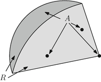
A is a set consisting of the dark crescent along with three isolated points. R consists of the dark and light regions and is the convex hull of A.
-
Ellipsoid: A Euclidean ellipsoid \(R \subset \mathbb{R}^{n}\) centered at \(x_{c} \in \mathbb{R}^{n}\) can be written as:
$$\displaystyle{ R =\Big\{ x_{c} + Au\Big\vert \vert \vert u\vert \vert _{2} \leq 1\Big\} }$$(18)with \(u \in \mathbb{R}^{n}\) and \(A \in \mathbb{R}^{n\times n}\) and non-singular.
-
Hyperplanes and halfspaces: Take \(x \in \mathbb{R}^{n}\), \(a \in \mathbb{R}^{n}\) and \(b \in \mathbb{R}\). A hyperplane \(R \subset \mathbb{R}^{n}\) can be defined as the set of points
$$\displaystyle{ R =\Big\{ x\Big\vert a'x = b,\quad a\neq 0\Big\} }$$(19)for some a and b. Similarly, a halfspace can be written as the set of points
$$\displaystyle{ R =\Big\{ x\Big\vert a'x \leq b,\quad a\neq 0\Big\}. }$$(20)for some a and b.
-
Convex polytope: Take \(x \in \mathbb{R}^{n}\), \(b \in \mathbb{R}^{m}\), and \(A \in \mathbb{R}^{m\times n}\). As discussed in the linear programming section, a convex polytope \(R \subset \mathbb{R}^{n}\) is the set of points:
$$\displaystyle{ R =\Big\{ x\Big\vert Ax \geq b\Big\}. }$$(21)

Convex sets have many important properties, but perhaps the most important is that the intersection of (even countably many) convex sets is convex. This fact ensures that adding more convex constraints will still result in a convex program.
3.2 Convex Functions
A function \(f: \mathbb{R}^{n} \rightarrow \mathbb{R}\) is convex if its domain is a convex set and:
Further, f is strictly convex if its domain is a convex set and:
Clearly, all strictly convex function are convex, but the reverse is not true. The graphical interpretation follows directly from the definition and is illustrated through Figures 4 and 5.

f(t) is a strictly convex function. For any x,y in the domain of f(t), the line segment connecting f(x) and f(y) is strictly above the function f(t) on x < t < y.

f(t) is a convex, but not strictly convex function. For any x,y the line segment connecting f(x) and f(y) is strictly above the function f(t) on x < t < y; however this is not the case for x and z, where the line segment connecting f(x) and f(z) lies directly on the function f(t).
Some examples of convex functions follow.
-
Linear-affine: f(x) = ax + b on \(\mathbb{R}\) for any \(a,b \in \mathbb{R}\)
-
Exponential: e ax on \(\mathbb{R}\) for any \(a \in \mathbb{R}\)
-
Power: x a on x > 0 for a ≥ 1 or a ≤ 0
-
Negative logarithm: − log(ax) on x > 0 for a > 0
If a function f is twice differentiable with open domain D, then it is convex if and only if
Here \(x \in \mathbb{R}^{n}\) and ∇2 f(x) denotes the Hessian
and “ ≥ ” is meant in the sense of a generalized inequality; in this case, that ∇2 f(x) is positive semi-definite (psd) (Figure 6).

A convex function \(f: \mathbb{R}^{2} \rightarrow \mathbb{R}\). The feasible region is R; the minimum of f over R is x ∗.
We can also show that f is convex if it can be obtained from simple convex functions by convexity-preserving operations, such as
-
Nonnegative weighted sum of convex functions
-
Pointwise maximum of convex functions
-
Composition of convex functions
3.3 Classes of Convex Programs
Many solvers take advantage of certain structural properties of the convex program in question. Here we list some important classes of convex programs seen in applications.
-
Linear program (LP): A linear objective function subject to linear equality and inequality constraints; the feasible region is a convex polytope. Discussed previously.
-
Quadratic program (QP): A quadratic objective function subject to linear equality and inequality constraints; the feasible region is therefore still a convex polytope. The general form of a QP is:
$$\displaystyle{ \begin{array}{rl} \min &\frac{1} {2}x'Px + q'x + r\\ \text{subject to} &Gx \leq h, \quad Ax = b \end{array} }$$(26)where the decision variable is \(x \in \mathbb{R}^{n}\), P is a psd matrix: \(P \in \mathbb{S}_{+}^{n}\), \(q \in \mathbb{R}^{n}\), and \(r \in \mathbb{R}^{n}\). Here we have explicitly separated the inequality constraints and equality constraints; the m inequality constraints are contained within Gx ≤ h where \(G \in \mathbb{R}^{m\times n}\) and \(h \in \mathbb{R}^{m}\). The p equality constraints are contained within Ax = b where \(A \in \mathbb{R}^{p\times n}\) and \(b \in \mathbb{R}^{p}\). P is required to be psd in order for the objective function to be convex, as ∇2(x′Px + q′x + r) = P.
Exercise 2.
Least-squares optimization
Formulate the linear least-squares approximation problem in n variables with m > n data points as a QP.
Solution 2.
If A is an m × n matrix containing the input data points and b is a m × 1 vector containing the output data points, then the problem is:
The objective function here is quadratic in x, so we must show that A′A is psd. A square matrix \(M \in \mathbb{R}^{p\times p}\) is psd if x′Mx ≥ 0 for all \(x \in \mathbb{R}^{p}\). For any x, we have
Thus, A is psd and so the objective function is convex. Furthermore, the constraints are trivially linear as there are none. Therefore, this is a QP. We can thus also consider the constrained least-squares problem, in which values of x must lie in an interval l ≤ x ≤ u; it is also a QP:
Exercise 3.
Portfolio optimization This example is from section 4.7.6 of Boyd and Vandenberghe [4]. Consider the problem of optimizing two criteria in assembling a financial portfolio: maximize the mean return and minimize the variance of the return. Let x be a vector containing the fractions of each of four possible assets. Each asset’s mean and standard deviation of return is given as:
Furthermore, the correlation coefficients between assets are: ρ 12 = 30% and ρ 13 = −40%; other pairs zero. Thus, the correlation matrix Σ is:
We define the mean return vector to be p: \(p = \left [\begin{array}{cccc} 0.12,&0.1,&0.07,&0.3 \end{array} \right ]'\), and we define a scaling factor μ that accounts for the relative importance of minimizing the variance of the return against maximizing the mean return. Formulate the problem as a quadratic program and solve.
Solution 3.
The problem is formulated as:
Here 1 represents a vector the same length as x with all entries being 1. Due to the form of the objective function, this is a quadratic program with linear constraints. The solution for various values of μ is graphed below, showing explicitly the tradeoff between the standard deviation of return versus the mean return (Figure 7).

Tradeoff between standard deviation and mean of the return.
Research Project 5.
Chapter 16 of Nocedal and Wright [11] delves into algorithms for QPs. Similar to the Simplex method, looking deeper into the run time of these algorithms for sample problems could provide an avenue to more theoretical projects.
-
Quadratically-constrained quadratic program (QCQP): A quadratic objective function subject to convex quadratic constraints. The general form of a QCQP is:
$$\displaystyle{ \begin{array}{rl} \min &\frac{1} {2}x'P_{0}x + q_{0}'x + r_{0} \\ \text{subject to}&\frac{1} {2}x'P_{i}x + q_{i}'x + r_{i} \leq 0,\quad i = 1,\ldots,m\\ &Ax = b\\ \end{array} }$$(31)with \(P_{i} \in \mathbb{S}_{+}^{n}\quad \forall \quad i = 0,\ldots,m\).
-
Second-order cone program (SOCP): A linear objective function subject to so-called second-order cone constraints. The general form of a SOCP is:
$$\displaystyle{ \begin{array}{rl} \min &f'x \\ \text{subject to}&\vert \vert A_{i}x + b_{i}\vert \vert _{2} \leq c_{i}'x + d_{i},\quad i = 1,\ldots,m \\ &Fx = G\\ \end{array} }$$(32)with \(A_{i} \in \mathbb{R}^{n_{1}\times n}\) and \(F \in \mathbb{R}^{p\times n}\). SOCPs are a generalization of QCQPs and LPs. QCQPs can be turned into SOCPs by reformulating the objective function as a constraint.
Research Project 6.
One problem from the area of robotics and optimal control is grasping a rigid body with robot fingers. To do so, we must determine the amount of force each finger shall exert. Lobo et al. [9] describe a formulation of this problem as a SOCP which takes into account friction and equilibrium constraints and limits on contact forces. We may simply be interested in whether the object can be grasped at all: this amounts to a feasibility problem, where we simply determine whether or not the feasible region is non-empty. If a solution does exist, we can investigate a variety of problems, such as finding the gentlest grip in some sense, or finding a grip which has the smallest difference in forces on each finger. Formulate the problem with a given number of fingers and a given object. This problem could also incorporate data-gathering, namely the physical properties of the object to be grasped.
Research Project 7.
Section 8.8 of Boyd and Vandenberghe [4] describes a floor-planning problem, where we seek the minimum perimeter fence to bound a set of rectangular objects of known dimension. Variants of the problem, including having a minimum spacing between the objects and allowing the dimensions (but not area) of the objects to vary, are considered. These can be formulated as SOCPs (where the | | ⋅ | |2 constraint corresponds to a Euclidean distance) or in some cases even LPs depending on the variant. Using this as a starting point, optimal packing problems can be considered for boxes or other shapes. This application has uses in shipping and transport problems.
-
Semi-definite program (SDP): One general form of an SDP is:
$$\displaystyle{ \begin{array}{rl} \min &c'x\\ \text{subject to} &x_{ 1}F_{1} + x_{2}F_{2} +\ldots +x_{n}F_{n} + G \geq 0 \\ &Ax = b\\ \end{array} }$$(33)with \(F_{i},G \in \mathbb{S}^{k},i = 1,2,\ldots,n\). The first constraint is known as a linear matrix inequality (LMI) constraint; since the left hand side is a k × k matrix, the “ ≥ ” here is a generalized inequality meaning that x 1 F 1 + x 2 F 2 + … + x n F n + G is psd. If F 1, …, F n , G are all diagonal, then this formulation reduces to a linear program. SDPs are a generalization of SOCPs, as the SOCP constraints can be written as LMIs.
Research Project 8.
Weinberger and Saul have formulated learning algorithms with applications to image processing as SDPs. Such algorithms can recognize characters in handwritten text, or identify whether faces from different image are the same person’s, even from different angles. Projects could be developed to identify a range of objects in images[14, 15].
Research Project 9.
An abundance of SDP applications can be found in the “Handbook of Semidefinite Programming” by Wolkowicz, Saigal, and Vandenberghe [16]. Projects could involve extending these applications and/or formulating new problems as SDPs.
3.4 Solvers
Many software packages exist to solve convex problems. One convenient solver for solving convex problems of moderate size (including LPs) is CVX, [5] which can be downloaded and used as a Matlab®; package. Other solvers include Gurobi [6] and CPLEX, [7] all of which are free for academic use, as well as Matlab’s Optimization ToolboxTM [10].
4 Concluding Remarks
Optimization is a powerful tool for solving many applied problems of interest to operations research. In this brief chapter we discussed linear programming, followed by the more general convex programming and specific forms therein. Many of these classes of problems have efficient algorithms for their solution, even in high dimensions; thus, formulation of an optimization problem in one of these forms often results in greatly improved computational tractability. For the undergraduate student, there are many open problems that are application-based. In addition, delving into the inner workings of algorithms for generic problems could provide an avenue to interesting projects.
4.1 Further Reading
Parts of this chapter were adapted from the textbooks “Introduction to Linear Optimization” by Bertsimas and Tsitsiklis, [2] and “Convex Optimization” by Boyd and Vandenberghe [4]. Another comprehensive text is Nocedal and Wright’s “Numerical Optimization.” [11].
References
Adler, I., Megiddo, N., Todd, M.J.: New results on the average behavior of simplex algorithms. Bull. Am. Math. Soc. 11(2), 378–382 (1984)
Bertsimas, D., Tsitsiklis, J.N.: Introduction to Linear Optimization. Athena Scientific, Belmont (1997)
Bosch, R.A.: The battle of the burger chains: which is best, burger king, mcdonald’s, or wendy’s? Socio Econ. Plan. Sci. 30(3), 157–162 (1996)
Boyd, S., Vandenberghe, L.: Convex Optimization. Cambridge University Press, Cambridge (2004)
Grant, M., Boyd, S.: CVX: Matlab software for disciplined convex programming, version 2.1. http://cvxr.com/cvx, Mar (2014)
Gurobi optimization. http://www.gurobi.com/products/gurobi-optimizer
IBM ILOG cplex optimization studio community edition. https://www-01.ibm.com/software/websphere/products/optimization/cplex-studio-community-edition
Klee, V., Minty, G.J.: How Good is the Simplex Algorithm? Defense Technical Information Center (1970)
Lobo, M.S., Vandenberghe, L., Boyd, S., Lebret, H.: Applications of second-order cone programming. Linear Algebra Appl. 284, 193–228 (1998)
MathWorks.: Matlab optimization toolbox. http://www.mathworks.com/products/optimization
Nocedal, J., Wright, S.J.: Numerical Optimization, 2nd edn. Springer, Berlin (2006)
Shamir, R.: The efficiency of the simplex method: a survey. Manag. Sci. 33(3), 301–34 (1987)
Smale, S.: Mathematical problems for the next century. Math. Intell. 20(2), 7–15 (1998)
Weinberger, K.Q., Saul, L.K.: Unsupervised learning of image manifolds by semidefinite programming. Proc. 2004 IEEE Computer Society Conference on Computer Vision and Pattern Recognition (2004)
Weinberger, K.Q., Saul, L.K.: Distance metric learning for large margin nearest neighbor classification. Machine Lear. Res. 10, 207–244 (2009)
Wolkowicz, H., Saigal, R., Vandenberghe, L. (eds.): Handbook of Semidefinite Programming. Kluwer Academic Publishers, Boston (2000)
Author information
Authors and Affiliations
Corresponding author
Editor information
Editors and Affiliations
Rights and permissions
Copyright information
© 2017 Springer International Publishing AG
About this chapter

Cite this chapter
Kotas, J. (2017). Mathematical Decision-Making with Linear and Convex Programming. In: Wootton, A., Peterson, V., Lee, C. (eds) A Primer for Undergraduate Research. Foundations for Undergraduate Research in Mathematics. Birkhäuser, Cham. https://doi.org/10.1007/978-3-319-66065-3_8
Download citation
DOI: https://doi.org/10.1007/978-3-319-66065-3_8
Published:
Publisher Name: Birkhäuser, Cham
Print ISBN: 978-3-319-66064-6
Online ISBN: 978-3-319-66065-3
eBook Packages: Mathematics and StatisticsMathematics and Statistics (R0)