Electrical Power Systems

Abstract

The general description of architecture and classification of power systems are presented at the beginning of the first chapter. Afterwards the basic concepts and analysis methods of electrical power systems are given, being accompanied by many examples of calculation. Also the power flow between the generators and consumers has been considered. In order to characterize the parameters of power systems next section of the first chapter is dedicated to measurement methods of power systems parameters. Electrical energy needed to power industrial or household electric consumers, like any other product, should satisfy specific quality requirements. In this respect the power quality aspects and the standards for power systems parameters are presented. The flow of reactive power and energy in power systems produces significant effects on the optimal functioning of suppliers and customers which are connected. Therefore in the last section of first chapter is defined the importance of reactive power in AC power systems and on its various understandings. Usually the first chapter is closed with a large list of bibliographic references.

These keywords were added by machine and not by the authors. This process is experimental and the keywords may be updated as the learning algorithm improves.

1 Chapter Overview

First part of this chapter is dedicated to an overview over all the topics presented in its sections. Power generation, transmission and distribution systems—that can be usually called electrical power systems —use almost exclusively AC circuits due to economic and technical advantages they offer. In this respect the second section of this chapter makes a general description of power systems. Generalities about the linear AC circuits in steady state conditions when the parameters as currents through and the voltages across the branches of circuits are sinusoidal are described in section three. Also the flow of power between generator and customers is studied by using the active, reactive, apparent and complex power like other important energetically parameters of AC circuits in sinusoidal state.

In the complex and interconnected power system a large variety of the electromagnetic field occurrences are present. They influence, in any time and location, the system parameters particularly his currents and voltages, one of the most important parameters being the power quality (PQ). Therefore all those who are interconnected and use the power system like power suppliers, distributors and customers are interested to preserve the PQ quality in their nominal values or in other words the electrical power as clean as possible.

Generally speaking the power quality term includes all the parameters which are defined for power systems. In order to check the PQ state, the parameters of power systems must be measured as accurately as possible. Herein in Sect. 4 of the chapter is presented an overview of the most important measurement and instrumentation methods of power systems parameters. In addition the parameters of PQ must be compared with a set of nominal (technical reference) values, namely standards. Particularly each country holds its own PQ standards and PQ instrumentation. On the other hand the globalization of the energy generation, transmission and market imposes general standards for common PQ parameters. A review of these international standards represents another purpose of this chapter which is allocated in Sect. 5.

The circulation of reactive power in power systems produces significant effects on the optimal functioning of suppliers and customers which are connected. Therefore about the importance of reactive power in AC power systems and on its various understandings refers the last section of the chapter.

This chapter is closed with a specific list of bibliographic references.

2 Introduction in Electrical Power Systems

Nowadays electrical power, together with natural resources, is becoming one of the most technical, economic and political factors. Often the stability and development of a region of the world depends on the respective countries’ energy systems and resources among which the electricity plays a key role.

The traditional architecture of Electrical Power Systems (EPS) is based on power generation, transmission, distribution and usage interconnected subsystems [1, 2]. For the past century the rate of change about energy production, distribution and customers is significant: on one hand the depletion of natural resources and environmental protection measures have led to the use of renewable energy sources (RES) such as wind turbines (WT), photovoltaic (PV) modules, geo-thermal (GT) or bio-mass (BM) systems and to the penetration of sophisticated distributed generation (DG) and Micro and Smart Grids (MG) systems; on the other hand through the development of industry production is resulted diverse range of much sensitive industrial and residential equipment [3, 4].

More efficient operation modes of distribution subsystems have been implemented with the increasing of DG penetration rate. Thus the presence of a multitude of energy sources leads to improving the continuity of power supply to the industrial and residential consumers. One the other hand there are several technical and economic issues that can be exceeded by introducing of new operation and control concepts as MG paradigm. The MG is a complex flexible and system control system of power flow between the generators and consumers. MG provides real-time decisions and auxiliary services to networks (relieves congestions, aiding restoration after faults e.a.). Also MG can provide to customers their thermal and electric energy needs, enhance the PQ, reduce the pollution and the costs of consumed energy e.a.

Nowadays complex and complicated technical, economic and political processes of industry and residential consumers development influence the dynamics of EPS [5,6,7]:

• globalization means the inter-country or inter-continental networks integration, energy market and investment combination and technological integration;

• liberalization is associated with the development of regional or inter-regional energy markets;

• decentralization assumes the development of small and large units power, together with upgrading and renewal of transmission and distribution networks, and introducing of DG concept;

• diversification means the increasing of multitude of energy sources (fuels, renewable energy sources e.a.) and of types of power plants;

• modernization results from the development of old technologies and the implementation of new and efficient ones.

Considering that EPS have different functions and nominal voltages, respectively various constructive types, there are some criteria for their classification [8,9,10]:

• criteria of nominal voltage is important because with its help is determine the power and distance that can be transmitted, the cost of the transmission line and its equipment e.a. EPS classification taking into account the nominal voltage is presenting in Table 1.1.

  Table 1.1 Classification of EPS

The nominal voltage means the rms value of a line voltage between phases; its standardized values are recommended by the International Electrotechnical Commission (CEI). For example the standardization values in kV are: 3; 3.3; 6; 10; 11; 15; 20; 22; 30; 45; 47; 66; 69; 110; 115; 132; 138; 150; 161; 220; 230; 287; 330; 345; 380; 400; 500; 700, and each country can adopt specific several such values. The LV is used in indoor electrical installations to supply directly the low voltage customers as well as the small urban and industrial networks, with power up to tens of kVA. The MV is used in urban and industrial networks for supply transformers with powers between tens and hundreds of kVA and also can supply directly medium voltage equipment. Transmission and distribution lines for powers between tens of MVA and 1–2 hundreds of MVA are carried out with HV. The VHV is used for transmission lines of powers between hundreds and thousands of MVA.

• criteria of functions classify EPS in usage (utilization), distribution and transmission networks.

• criteria of topology classify EPS in: (i) radial networks that means each customer can be supplied from one side (source) only; (ii) meshed networks that means each customer can be supplied from two sides; (iii) complex meshed networks that means each customer can be supplied from of more than the two sides.

• criteria of adopted power system classify EPS in AC respectively DC. Starting from historical scientific insights of M. Dolivo-Dobrovolski and N. Tesla now the widespread EPS system consists in 3 and 2-phases electrical AC networks. But from struggle between AC and DC transmission systems is possible in the near future that very high voltage DC systems to win.

3 Basic Concepts and Analysis Methods of Electrical Power Systems

From theoretical point of view EPS are considering as symmetrical three-phase systems, condition that is ensured through the symmetrization of transmissions and distribution lines, and transformers. Starting from this ideal assumption the symmetrical three-phase transmission and distribution networks, including equipment and transformers, can be analyzed by using symmetrical components method and the decomposition in single phase circuits. The equivalent circuits of EPS contain non-linear passive elements, as resistances, inductances and capacitances. Nonlinearity of these elements are neglected in most frequent calculations, considering that their values change relatively small according to the low and expected limits of change of the voltage, current or frequency. For this reason the equivalent circuits of EPS are considered linear and are disposed longitudinal and transversal as in Γ, T or Π scheme types [11,12,13].

A three-phase symmetrical and positive phase-sequence system in instantaneous values is expressed as [14, 15]

$$ \begin{aligned} & v_{d1} (t) = V\sqrt 2 \sin (\omega t + \gamma ) \\ & v_{d2} (t) = V\sqrt 2 \sin (\omega t + \gamma - \frac{2\pi }{3}) \\ & v_{d3} (t) = V\sqrt 2 \sin (\omega t + \gamma - \frac{4\pi }{3}) = V\sqrt 2 \sin (\omega t + \gamma + \frac{2\pi }{3}) \\ \end{aligned} $$

(1.1)

respectively by the complex vectors

$$ \begin{aligned} & \underline{V}_{d1} = Ve^{j\gamma } = \underline{V} \\ & \underline{V}_{d2} = Ve^{{j(\gamma - \frac{2\pi }{3})}} = \underline{V} e^{{ - j\frac{2\pi }{3}}} = a^{2} \underline{V} \\ & \underline{V}_{d3} = Ve^{{j(\gamma + \frac{2\pi }{3})}} = \underline{V} e^{{j\frac{2\pi }{3}}} = a\underline{V} \\ \end{aligned} $$

(1.2)

where $a = e^{{j\frac{2\pi }{3}}} = e^{{ - j\frac{4\pi }{3}}} = - \frac{1}{2} + j\frac{\sqrt 3 }{2}$ is called phase operator. The representation of instantaneous values (1.1) in time domain and of complex vectors (1.2) in complex Cartesian coordinates are presented in Fig. 1.1a, b.

Fig. 1.1

Representation of three-phase symmetrical and positive phase-sequence system: a Time domain, b Cartesian coordinates

A three-phase symmetrical and negative phase-sequence system in instantaneous values is expressed as

$$ \begin{aligned} & v_{i1} (t) = V\sqrt 2 \sin (\omega t + \gamma ) \\ & v_{i2} (t) = V\sqrt 2 \sin (\omega t + \gamma + \frac{2\pi }{3}) \\ & v_{i3} (t) = V\sqrt 2 \sin (\omega t + \gamma - \frac{2\pi }{3}) \\ \end{aligned} $$

(1.3)

respectively by the complex vectors

$$ \begin{aligned} & \underline{V}_{i1} = Ve^{j\gamma } = \underline{V} \\ & \underline{V}_{i2} = Ve^{{j(\gamma + \frac{2\pi }{3})}} = \underline{V} e^{{j\frac{2\pi }{3}}} = a\underline{V} \\ & \underline{V}_{i3} = Ve^{{j(\gamma - \frac{2\pi }{3})}} = \underline{V} e^{{ - j\frac{2\pi }{3}}} = a^{2} \underline{V} \\ \end{aligned} $$

(1.4)

which have the representations in time domain and complex Cartesian coordinates illustrated in Fig. 1.2a, b.

Fig. 1.2

Representation of three-phase symmetrical and negative phase-sequence system: a Time domain, b Cartesian coordinates

A three-phase symmetrical and zero phase-sequence system in instantaneous values is expressed as

$$ v_{01} (t) = v_{02} (t) = v_{03} (t) = V\sqrt 2 \sin (\omega t + \gamma ) $$

(1.5)

and by the complex vectors

$$ \underline{V}_{o1} = \underline{V}_{o2} = \underline{V}_{o3} = Ve^{j\gamma } = \underline{V} $$

(1.6)

The representation of values (1.5) and (1.6) is shown in Fig. 1.3a, b.

Fig. 1.3

Representation of three-phase symmetrical and zero phase-sequence system: a Time domain, b Cartesian coordinates

Practically, two general connections are considered in EPS: star and delta [16,17,18].

• (i) Star connection. Let us consider an elementary EPS in which the generator (G) and consumer (load, receptor—R) are arranged into a star connection. The transmission line (L) links G with R. The star connection illustrated in Fig. 1.4 is defined in that all the phase terminals are connected together to form the neutral point. The both neutral nodes of the generator “O” and of the receptor “N” is linked by neutral wire. The electromotive voltages of generators e ₁, e ₂, e ₃, the voltages across the terminals of generators $u_{{1_{G} }} , \, u_{{2_{G} }} , \, u_{{3_{G} }}$, the voltages between the transmission lines u ₁₂, u ₂₃, u ₃₁, the currents in the transmission lines i ₁, i ₂, i ₃ and the voltages across the terminals of receptor $u_{{1_{R} }} , \, u_{{2_{R} }} , \, u_{{3_{R} }}$ there are three-phase systems.

  Fig. 1.4

  

  Star connection

For an adequate systematization of knowledge following definitions are useful:

• the triplets $\left( {e_{1} , \, u_{{1_{G} }} , \, i_{{1_{G} }} } \right)$, $\left( {e_{2} , \, u_{{2_{G} }} , \, i_{{2_{G} }} } \right)$ and $\left( {e_{3} , \, u_{{3_{G} }} , \, i_{{3_{G} }} } \right)$ are called phase signals of generators;

• the doublets $\left( {u_{{1_{R} }} , \, i_{{1_{R} }} } \right)$, $\left( {u_{{2_{R} }} , \, i_{{2_{R} }} } \right)$ and $\left( {u_{{3_{R} }} , \, i_{{3_{R} }} } \right)$ are called phase signals of receptors (consumers);

• the voltages (u ₁₂, u ₂₃, u ₃₁) between of the three line wires are called line voltages, also the line impedances have not been taken into account;

• the currents (i ₁, i ₂, i ₃) across the line wires are called line currents;

• the impedances Z ₁ , Z ₂, Z ₃ are called phase impedances of receptor.

Generally speaking the set signals $\left( {e_{1} , \, u_{{1_{G} }} , \, i_{{1_{G} }} ,u_{{1_{R} }} , \, i_{{1_{R} }} ,\underline{Z}_{1} } \right)$ makes up phase 1 of star connection and similar definitions are used for the other two phases. For star connection the line currents are equal to the phase currents

$$ i_{1G} = i_{1} = i_{1R} ; \, i_{2G} = i_{2} = i_{2R} ; \, i_{3G} = i_{3} = i_{3R} $$

(1.7)

respectively in complex values

$$ \underline{I}_{1G} = \underline{I}_{1} = \underline{I}_{{1_{R} }} ; \, \underline{I}_{2G} = \underline{I}_{2} = \underline{I}_{{2_{R} }} ; \, \underline{I}_{3G} = \underline{I}_{3} = \underline{I}_{{3_{R} }} \, $$

(1.8)

and in rms values I _l  = I _ph .

Also for the neutral wire are defined: i ₀ or i _n —the current, u _NO or u _n —the voltage, and Z ₀ or Z _N —the impedance.

Considering the positive reference directions for line currents from generators to receptors and for current across the neutral wire from neutral point of the receptors to that of the generators, then by applying Kirchhoff laws following relations in complex values are described the star connection

$$ \begin{aligned} & \underline{I}_{1} + \underline{I}_{2} + \underline{I}_{3} = \underline{I}_{0} \\ & \underline{U}_{12} = \underline{U}_{{1_{R} }} - \underline{U}_{{2_{R} }} \\ & \underline{U}_{23} = \underline{U}_{{2_{R} }} - \underline{U}_{{3_{R} }} \\ & \underline{U}_{31} = \underline{U}_{{3_{R} }} - \underline{U}_{{1_{R} }} \\ & \underline{U}_{12} + \underline{U}_{23} + \underline{U}_{31} = 0 \\ & \underline{U}_{{1_{R} }} + \underline{U}_{NO} + \underline{U}_{10} = 0 \\ & \underline{U}_{{2_{R} }} + \underline{U}_{NO} + \underline{U}_{20} = 0 \\ & \underline{U}_{{3_{R} }} + \underline{U}_{NO} + \underline{U}_{30} = 0 \\ \end{aligned} $$

(1.9)

Another set of relations express Ohm’s law for receptor phases and for neutral wire in complex values are expressed as

$$ \begin{aligned} & \underline{U}_{{1_{R} }} = \underline{Z}_{1} \cdot \underline{I}_{1} \\ & \underline{U}_{{2_{R} }} = \underline{Z}_{2} \cdot \underline{I}_{2} \\ & \underline{U}_{{3_{R} }} = \underline{Z}_{3} \cdot \underline{I}_{3} \\ & \underline{U}_{NO} = \underline{Z}_{0} \cdot \underline{I}_{0} \\ \end{aligned} $$

(1.10)

• (ii) Delta connection. Let us consider an elementary EPS in which the generator and receptor (consumer) are arranged into a delta (mesh) connection (Fig. 1.5). The transmission line links generator with receptor. Symmetrical cycling between the pairs of impedances leads so that the start terminal of one phase impedance is connected to the finish terminal of another are used for delta connection.

  Fig. 1.5

  

  Delta connection

For an adequate systematization of knowledge following definitions are useful:

• the triplets $\left( {e_{12} , \, u_{{21_{G} }} , \, i_{{21_{G} }} } \right)$, $\left( {e_{23} , \, u_{{23_{G} }} , \, i_{{23_{G} }} } \right)$ and $\left( {e_{31} , \, u_{{31_{G} }} , \, i_{{31_{G} }} } \right)$ are called phase signals of generators;

• the doublets $\left( {u_{{12_{R} }} , \, i_{{12_{R} }} } \right)$, $\left( {u_{{23_{R} }} , \, i_{{23_{R} }} } \right)$ and $\left( {u_{{31_{R} }} , \, i_{{31_{R} }} } \right)$ are called phase signals of receptors (consumers);

• the voltages (u ₁₂, u ₂₃, u ₃₁) between of the three line wires are called line voltages, also the line impedances have not been taken into account;

• the currents (i ₁, i ₂, i ₃) across the line wires are called line currents;

• the impedances Z ₁₂ , Z ₂₃, Z ₃₁ are called phase impedances of receptor.

Generally speaking the set signals $\left( {e_{12} , \, u_{{12_{G} }} , \, i_{{12_{G} }} ,u_{{12_{R} }} , \, i_{{12_{R} }} ,\underline{Z}_{12} } \right)$ makes up phase 1 of delta connection and similar definitions are used for the other two phases. If the line impedances are not considering, for star connection the line voltages of generators are equal to the line voltage of receptor

$$ u_{{12_{G} }} = u_{{12_{R} }} = u_{12} ,u_{{23_{G} }} = u_{{23_{R} }} = u_{23} ,u_{{31_{G} }} = u_{{31_{R} }} = u_{31} $$

(1.11)

and in rms values V _l  = V _ph .

Based on Kirchhoff’s current law (KCL) the following relations are true

$$ \begin{aligned} & \underline{I}_{1} = \underline{I}_{12} - \underline{I}_{31} \\ & \underline{I}_{2} = \underline{I}_{23} - \underline{I}_{12} \\ & \underline{I}_{3} = \underline{I}_{31} - \underline{I}_{23} \\ \end{aligned} $$

(1.12)

By summing (1.12) results

$$ \underline{I}_{1} + \underline{I}_{2} + \underline{I}_{3} = 0 $$

(1.13)

Also applying Ohm’s law on each phase of the receptor are obtained

$$ \begin{aligned} & \underline{U}_{12} = \underline{Z}_{12} \cdot \underline{I}_{12} \\ & \underline{U}_{23} = \underline{Z}_{23} \cdot \underline{I}_{23} \\ & \underline{U}_{31} = \underline{Z}_{31} \cdot \underline{I}_{31} \\ \end{aligned} $$

(1.14)

A three-phase system is called symmetrical if it is supplied by a symmetrical voltages system (1.1), (1.3) or (1.5). Otherwise it is considered unsymmetrical. If all the complex phase impedances of star or delta connection are equal the system is balanced, otherwise is non-balanced. A symmetrical and balanced system produces symmetrical lines and phases currents systems. In symmetrical and balanced systems all neutral points are the same potential and the current across the neutral wire is null. On the other hand in symmetrical and balanced conditions for star connection the rms value of line voltage is $\sqrt 3$ times the rms value of phase voltage $V_{l} = \sqrt 3 V_{ph}$, respectively for delta connection the rms value of line current is $\sqrt 3$ times the rms value of phase current $I_{l} = \sqrt 3 I_{ph}$.

The overall complex powers absorbed by a receptor in star (including the neutral wire) and delta connections are given by

$$ \begin{aligned} \underline{S}_{{_{R,star} }} & = \underline{U}_{{1_{R} }} \underline{I}_{1}^{*} + \underline{U}_{{2_{R} }} \underline{I}_{2}^{*} + \underline{U}_{{3_{R} }} \underline{I}_{3}^{*} + \underline{U}_{NO} \underline{I}_{0}^{*} = \underline{Z}_{1} I_{1}^{2} + \underline{Z}_{2} I_{2}^{2} + \underline{Z}_{3} I_{3}^{2} + \underline{Z}_{0} I_{0}^{2} \\ & = P_{R,star} + jQ_{R,star} \\ \end{aligned} $$

(1.15)

respectively

$$ \begin{aligned} \underline{S}_{{_{R,delta} }} & = \underline{U}_{{12_{R} }} \underline{I}_{12}^{*} + \underline{U}_{{23_{R} }} \underline{I}_{23}^{*} + \underline{U}_{{31_{R} }} \underline{I}_{31}^{*} = \underline{Z}_{12} I_{12}^{2} + \underline{Z}_{23} I_{23}^{2} + \underline{Z}_{31} I_{31}^{2} + \underline{Z}_{0} I_{0}^{2} \\ & = P_{R,delta} + jQ_{R,delta} \\ \end{aligned} $$

(1.16)

where the real part represents the overall active absorbed power (P _R —dissipated in the resistors) and the imaginary part represents the overall absorbed reactive power (Q _R —dissipated in the inductors minus in the capacitors). When symmetrical and balanced conditions are verified then for any form of interlinkage (star or delta) the overall active and reactive absorbed powers are given by

$$ \begin{aligned} & P_{R} = 3V_{ph} I_{ph}^{{}} \cos \varphi = \sqrt 3 V_{l} I_{l}^{{}} \cos \varphi \\ & Q_{R} = 3V_{ph} I_{ph}^{{}} \sin \varphi = \sqrt 3 V_{l} I_{l}^{{}} \sin \varphi \\ \end{aligned} $$

(1.17)

where the angle φ is the phase displacement between the voltage and current phases, or in other word, is the phase angle of the complex phase impedance. Also the apparent (overall) power for star and delta connections is defined as

$$ S_{R,star} = \sqrt {P_{R,star}^{2} + Q_{R,star}^{2} } ;\quad S_{R,delta} = \sqrt {P_{R,delta}^{2} + Q_{R,delta}^{2} } $$

(1.18)

According to the Eq. (1.17) in symmetrical and balanced conditions for both connections the following expression is true

$$ S_{R} = 3V_{ph} I_{ph} = \sqrt 3 V_{l} I_{l} $$

(1.19)

The calculation methods of EPS are based on the properties of three-phase circuits with different types of supplying system’s voltages and on some properties of various phase connections [19, 20]. Two elementary methods are presented below.

• (α) Calculation of symmetrical and balanced three-phase circuits. In this case we assume that the voltage generators are symmetrical and know, and also the receptor is balanced. Symmetrical three-phase circuits consisting of many star or delta receptors are solved by the use of single-phase circuit, for example of phase 1. Based on the principles of this elementary method have been developed software programs for the analysis of three-phase circuits. This method contains following steps [21, 22]:

• (α1) The coupled inductances in phase 1 are replaced with equivalent inductance −Z _m . Based on three-phase symmetrical currents property I ₁ + I ₂ + I ₃ = 0, then the voltage across the coupled inductance in phase 1 can be expressed as U _m,1 = Z _m I ₂ + Z _m I ₃ = Z _m (I ₂ + I ₃) = −Z _m I ₁, where the complex mutual impedance is Z _m  = $\pm$ jωM, and M is the mutual inductance which can be considered in aiding (+) or opposite (−) direction. Analogous equivalences are applied to couple inductances of other two phases.

• (α2) All the delta connections are replaced with equivalent star connections, by using the relation $\underline{Z}_{Y} = \underline{Z}_{\Delta } /3$, where Z _Y and Z _Δ are the phase impedances of star respectively delta connections.

• (α3) In a symmetrical and balanced three-phase star circuits all neutral points have the same potential and I ₁ + I ₂ + I ₃ = I _N  = 0. Therefore all neutral points can be connected each other through a null resistance wire without modifying the three-phase circuit voltages and currents. Such the single-phase circuit becomes a closed-loop.

• (α4) The voltages and currents of phase 1 are calculated by using the Kirchhoff’s laws in single-phase circuit. Finally on determine the other two phases voltages and currents through the use of phase operator a, according to the type of phase-sequences of the voltages generator system.

• (α5) By using Eqs. (1.17) and (1.19) the overall active, reactive, apparent and complex absorbed power are calculated.

Example 1.1

Let us consider a symmetrical three-phase generator in star connection shown in Fig. 1.6. Its positive phase-sequence voltages system are $\underline{E}_{1} = 400\sqrt 2$, $\underline{E}_{2} = 400\sqrt 2 e^{{ - j\frac{2\pi }{3}}} ,\underline{E}_{3} = 400\sqrt 2 e^{{ + j\frac{2\pi }{3}}}$ supplying through a transmission line impedance Z ₁ = 40 + 80j first star connection receptor R ₁ = 40 Ω, X _L1 = X _C1 = X _M1 = 40 Ω, neutral wire impedance Z _ON1 = 10(1−j) Ω, and through another transmission line impedance r ₁ = 10 Ω, the second delta connection receptor R ₂ = 90 Ω, X _L2 = 150 Ω and X _M2 = 30 Ω.

Fig. 1.6

Symmetrical and balanced three-phase system

In order to calculate the generator line currents (I ₁₁, I ₂₁, I ₃₁), the phase currents (I _1Y , I _2Y , I _3Y ) and voltages (U _1Y , U _2Y , U _3Y ) of star receptor, the phase currents (I _12Δ, I _23Δ, I _31Δ) and voltages (U _12Δ, U _23Δ, U _31Δ) of delta receptor and the overall absorbed powers, the above mentioned elementary method is applied:

• (α1) The equivalences of coupled inductances of star and delta connections are presented in Fig. 1.7;

  Fig. 1.7

  

  Equivalent three-phase circuit

• (α2) Replacement of delta connection with equivalent star connection whose neutral point is N₂ is shown in Fig. 1.8. There the values of equivalent impedances are

  Fig. 1.8

  

  Equivalence delta—star

  $$ \begin{aligned} \underline{Z}_{1Y} & = R_{1} + j(X_{L1} - X_{M1} - X_{C1} ) = 40(1 - j)\Omega \\ \underline{Z}_{{2Y_{e} }} & = \frac{{\underline{Z}_{2\Delta } }}{3} = \frac{{R_{2} + j(X_{L2} - X_{M2} )}}{3} = \frac{90 + 120j}{3} = 30 + 40j\Omega \\ \end{aligned} $$

• (α3) A null resistance wire is introduced in order to connect all the neutral points O, N and N₁ (dash line in Fig. 1.8);

• (α4) The single-phase circuit of phase 1 is shown in Fig. 1.9. By using Kirchhoff’s laws one obtains

  Fig. 1.9

  

  Single-phase circuit of phase 1

  $$ \underline{I}_{11} = \frac{{\underline{E}_{1} }}{{\underline{Z}_{1} + \frac{{\underline{Z}_{1Y} (r_{1} + \underline{Z}_{{2Y_{e} }} )}}{{\underline{Z}_{1Y} + r_{1} + \underline{Z}_{{2Y_{e} }} }}}} = 5e^{{ - j\frac{\pi }{4}}} {\text{ A}};\quad \underline{I}_{1Y} = \underline{I}_{11} \cdot \frac{{r_{e} + \underline{Z}_{1Ye} }}{{\underline{Z}_{1Y} + r_{e} + \underline{Z}_{2Ye} }} = \frac{5\sqrt 2 }{2} \, A $$

The currents of other two phases of first star receptor are obtained by using the phase operator

$$ \underline{I}_{2Y} = \underline{I}_{1Y} e^{{ - j\frac{2\pi }{3}}} = \frac{5\sqrt 2 }{2}e^{{ - j\frac{7\pi }{6}}} {\text{ A;}}\quad \underline{I}_{3Y} = \underline{I}_{1Y} e^{{j\frac{2\pi }{3}}} = \frac{5\sqrt 2 }{2}e^{{j\frac{\pi }{6}}} {\text{ A}} $$

From KCL results the line 1 current of the second equivalent star $\underline{I}^{\prime }_{11} = \underline{I}_{1Ye} = \frac{5\sqrt 2 }{2}e^{{ - j\frac{\pi }{2}}} {\text{A}}$. Then the other two phase currents are calculated as $\underline{I}_{21}^{{\prime }} = \underline{I}_{2Ye} = \underline{I}_{11}^{{\prime }} e^{{ - j\frac{2\pi }{3}}} = \frac{5\sqrt 2 }{2}e^{{ - j\frac{7\pi }{6}}} {\text{A,}}\quad \underline{I}_{31}^{{\prime }} = \underline{I}_{3Ye} = \underline{I}_{11}^{{\prime }} e^{{j\frac{2\pi }{3}}} = \frac{5\sqrt 2 }{2}e^{{j\frac{\pi }{6}}} {\text{A}}$.

If the properties of symmetrical systems are used thus the delta connection receptor is crossed by the phase currents

$$ \begin{aligned} \underline{I}_{12\Delta } & = \underline{I}_{1Ye} \sqrt 3 e^{{ - j\frac{\pi }{6}}} = \frac{5}{2}\sqrt 6 e^{{ - j\frac{2\pi }{3}}} {\text{A}},\quad \underline{I}_{23\Delta } = \underline{I}_{2Ye} \sqrt 3 e^{{ - j\frac{\pi }{6}}} = \frac{5\sqrt 6 }{2}e^{{ - j\frac{4\pi }{3}}} {\text{A}}, \\ \underline{I}_{31\Delta } & = \underline{I}_{3Ye} \sqrt 3 e^{{ - j\frac{\pi }{6}}} = \frac{5\sqrt 6 }{2}{\text{A}} \\ \end{aligned} $$

First star receptor has the phase voltages

$$ \begin{aligned} \underline{U}_{1Y} & = \underline{Z}_{1Y} \underline{I}_{1Y} = 200e^{{ - j\frac{\pi }{4}}} {\text{V}},\quad \underline{U}_{2Y} = \underline{U}_{1Y} e^{{ - j\frac{2\pi }{3}}} = 200e^{{ - j\frac{11\pi }{12}}} {\text{V}}, \\ \underline{U}_{3Y} & = \underline{U}_{1Y} e^{{j\frac{2\pi }{3}}} = 200e^{{j\frac{5\pi }{12}}} {\text{V}} \\ \end{aligned} $$

and also the phase voltages of delta receptor are given by

$$ \begin{array}{*{20}c} {\underline{U}_{12\Delta } = \underline{Z}_{1\Delta } \underline{I}_{12\Delta } = 375\sqrt 6 e^{{j\left( { - \frac{2\pi }{3} + \arctan \frac{4}{3}} \right)}} {\text{V}},\quad \underline{U}_{23\Delta } = \underline{U}_{12\Delta } e^{{ - j\frac{2\pi }{3}}} = 375\sqrt 6 e^{{j\left( { - \frac{4\pi }{3} + \arctan \frac{4}{3}} \right)}} } \\ {\text{V}} \\ {\underline{U}_{31\Delta } = \underline{U}_{12\Delta } e^{{j\frac{2\pi }{3}}} = 375\sqrt 6 e^{{j\left( {\arctan \frac{4}{3}} \right)}} {\text{V}}} \\ \end{array} $$

(α5) The overall absorbed active, reactive, apparent and complex powers by receptors and transmission lines are respectively

$$ \begin{aligned} P_{abs} & = 3\text{Re} \left[ {\underline{Z}_{e} } \right]\underline{I}_{11}^{2} + 3\text{Re} \left[ {\underline{Z}_{1y} } \right]\underline{I}_{1y}^{2} + 3r_{e} \underline{I}_{11}^{2} + 3\text{Re} \left[ {\underline{Z}_{2\Delta } } \right]\underline{I}_{12\Delta }^{2} = 6000{\text{ W}} \\ Q_{abs} & = 3\text{Im} \left[ {\underline{Z}_{1} } \right]\underline{I}_{11}^{2} + 3\text{Im} \left[ {\underline{Z}_{1y} } \right]\underline{I}_{1y}^{2} + 3\text{Im} \left[ {\underline{Z}_{2\Delta } } \right]\underline{I}_{12\Delta }^{2} = 6000{\text{ VAr}} \\ S_{abs} & = 3\left| {\underline{Z} } \right|_{1} \cdot \underline{I}_{11}^{2} + 3\left| {\underline{Z} } \right|_{1y} \cdot \underline{I}_{1y}^{2} + 3r_{e} \cdot \underline{I'}_{11}^{2} + 3\left| {\underline{Z} } \right|_{12\Delta } \cdot \underline{I}_{12\Delta }^{2} = \sqrt {P_{abs}^{2} + Q_{abs}^{2} } = 6000\sqrt 2 {\text{ VA}} \\ \underline{S}_{abs} & = P + jQ = 6000 + 6000j \\ \end{aligned} $$

These powers are received from the generator whose overall complex power is

$$ \underline{S}_{gen} = \underline{E}_{1} \underline{I}_{11}^{*} + \underline{E}_{2} \underline{I}_{21}^{*} + \underline{E}_{3} \underline{I}_{31}^{*} = 3\underline{E}_{1} \underline{I}_{11}^{*} = 6000 + 6000j $$

hence the conservation of active and reactive powers is proved

$$ P_{gen} = \text{Re} \left[ {\underline{S}_{gen} } \right] = 6000{\text{ W}} \equiv P_{abs} ; \, Q_{gen} = \text{Im} \left[ {\underline{S}_{gen} } \right] = 6000{\text{ VAr}} \equiv Q_{abs} $$

Due to the losses in transmission lines, the active power transmission efficiency can be calculated as

$$ \eta = \frac{{3\text{Re} [\underline{Z}_{ 1Y} ].\underline{I}_{1Y}^{2} + 3\text{Re} [\underline{Z}_{ 2\Delta } ].\underline{I}_{ 1 2\Delta }^{2} }}{{P_{abs} }} = 0.68 $$

Also the power factor (PF, also $\lambda$ or $\cos \varphi$) of the considered EPS is defined as

$$ \lambda = \cos \varphi = \frac{P}{S} = 0.706 $$

(β) Calculation of asymmetrical three-phase circuits by using the method of symmetrical components. In EPS two kinds of asymmetry transverse and longitudinal may occur. Transverse asymmetry occurs when an unbalanced receptor is connected to a symmetrical three-phase network. Such an unbalanced load may take the form of asymmetrical short-circuits as line-to-line, one or two line-to-earth short-circuits. Longitudinal asymmetry occurs when the phases of a transmission line contain un-equal impedances (unsymmetrical section of transmission line) or when an open-circuit occurs in one or two phases. By the elementary method of symmetrical components an asymmetrical three-phase set of currents or voltages can be decomposed into three symmetrical systems positive, negative and zero phase-sequence which are called symmetrical components [23]. Since it is based on superposition theorem the decomposition can be applied only to linear circuits.

It is demonstrates that any asymmetrical three-phase system $\underline{V}_{1} ,\underline{V}_{2} ,\underline{V}_{3}$ can be explained as the sum of three symmetrical systems: positive, negative and zero phase-sequences [24, 25], so

$$ \begin{aligned} \underline{V}_{1} = \underline{V}_{o1} + \underline{V}_{d1} + \underline{V}_{i1} \hfill \\ \underline{V}_{2} = \underline{V}_{o2} + \underline{V}_{d2} + \underline{V}_{i2} \hfill \\ \underline{V}_{3} = \underline{V}_{o3} + \underline{V}_{d3} + \underline{V}_{i3} \hfill \\ \end{aligned} $$

(1.20)

where

$$ \underline{V}_{d1} = \underline{V}_{d} \;,\;\underline{V}_{d2} = \underline{V}_{d} \cdot e^{{ - j\frac{2\pi }{3}}} = a^{2} \underline{V}_{d} \;,\;\underline{V}_{d1} = \underline{V}_{d} \cdot e^{{j\frac{2\pi }{3}}} = a\underline{V}_{d} $$

(1.21)

$$ \underline{V}_{i1} = \underline{V}_{i} \;,\;\underline{V}_{i2} = \underline{V}_{i} \cdot e^{{j\frac{2\pi }{3}}} = a \cdot \underline{V}_{i} \;,\;\underline{V}_{i1} = \underline{V}_{i} \cdot e^{{ - j\frac{2\pi }{3}}} = a^{2} \cdot \underline{V}_{i} $$

(1.22)

$$ \underline{V}_{o1} = \underline{V}_{o2} = \underline{V}_{o3} = \underline{V}_{o} $$

(1.23)

Taking into account the relations (1.21)–(1.23), the decomposition (1.21)—shown in Fig. 1.10—can be rewritten in the form

Fig. 1.10

Decomposition of an unsymmetrical system in three symmetrical systems

$$ \begin{aligned} & \underline{V}_{1} = \underline{V}_{o} + \underline{V}_{d} + \underline{V}_{i} \\ & \underline{V}_{2} = \underline{V}_{o} + a^{2} \cdot \underline{V}_{d} + a \cdot \underline{V}_{i} \\ & \underline{V}_{3} = \underline{V}_{o} + a \cdot \underline{V}_{d} + a^{2} \cdot \underline{V}_{i} \\ \end{aligned} $$

(1.24)

If it is considered know the asymmetrical system $\underline{V}_{1} ,\underline{V}_{2} ,\underline{V}_{3}$, then zero $(\underline{V}_{o} )$, positive $(\underline{V}_{d} )$ and negative-sequences $(\underline{V}_{i} )$ are calculated as

$$ \begin{aligned} & \underline{V}_{o} = \frac{1}{3}\left( {\underline{V}_{1} + \underline{V}_{2} + \underline{V}_{3} } \right) \\ & \underline{V}_{d} = \frac{1}{3}\left( {\underline{V}_{1} + a \cdot \underline{V}_{2} + a^{2} \cdot \underline{V}_{3} } \right) \\ & \underline{V}_{i} = \frac{1}{3}\left( {\underline{V}_{1} + a^{2} \cdot \underline{V}_{2} + a \cdot \underline{V}_{3} } \right) \\ \end{aligned} $$

(1.25)

In order to evaluate the state of asymmetry, are defined two dimensionless parameters: the coefficient of dissymmetry $\varepsilon_{d} = \frac{{V_{i} }}{{V_{d} }}$, and the coefficient of asymmetry $\varepsilon_{a} = \frac{{V_{o} }}{{V_{d} }}$, where $V_{o}$, $V_{d}$, $V_{i}$ are the rms values of zero, positive and negative-sequences. In real applications a system is considered symmetrical if $\varepsilon_{d}$ and $\varepsilon_{a}$ have values lower than 0.05.

The calculation of three-phase systems operating under asymmetrical conditions can be made based on the superposition theorem: are calculated separately each symmetrical component, and finally these components gather.

Example 1.2

Let us consider a balanced star receptor supplied by an asymmetrical system of phase voltages $\underline{U}_{10} ,\;\underline{U}_{20} ,\;\underline{U}_{30}$. The calculation of phase currents $\underline{I}_{1} ,\;\underline{I}_{2} ,\;\underline{I}_{3}$ is made by method of symmetrical components. Asymmetrical system shown in Fig. 1.11a, is decomposed in three symmetrical systems positive (Fig. 1.11b), negative (Fig. 1.11c) and zero-sequences (Fig. 1.11d).

Fig. 1.11

Decomposition of the a unsymmetrical system, b positive, c negative, and d zero-sequences

Since the receiver is balanced, the current through the neutral wire is zero for positive and negative component, and for zero-sequence component is 3 times the phase current because the phase currents are equal. The reducing of the system to a single phase is made by using the equivalent circuit shown in Fig. 1.12: single phase of positive (Fig. 1.12a), negative (Fig. 1.12a), and zero-sequence (Fig. 1.12c).

Fig. 1.12

Single phases of a positive, b negative, and c zero-sequence

Phase voltages corresponding to each circuit are respectively

$$ \underline{U}_{{d_{1} }} = \underline{Z} \cdot \underline{I}_{{d_{1} }} ;\quad \underline{U}_{{i_{1} }} = \underline{Z} \cdot \underline{I}_{{i_{1} }} ;\quad \underline{U}_{{o_{1} }} = \left( {\underline{Z} + 3\underline{Z}_{0} } \right) \cdot \underline{I}_{{o_{1} }} $$

(1.26)

The two other phase currents for positive and negative sequence are calculated by using the phase operator. Finally the phase currents of initial asymmetrical system are calculated by summing of symmetrical current components as

$$ \begin{aligned} & \underline{I}_{1} = \underline{I}_{{o_{1} }} + \underline{I}_{{d_{1} }} + \underline{I}_{{i_{1} }} = \frac{{\underline{U}_{{o_{1} }} }}{{\underline{Z} + 3\underline{Z}_{0} }} + \frac{{\underline{U}_{{d_{1} }} }}{{\underline{Z} }} + \frac{{\underline{U}_{{i_{1} }} }}{{\underline{Z} }} \\ & \underline{I}_{2} = \underline{I}_{{o_{2} }} + \underline{I}_{{d_{2} }} + \underline{I}_{{i_{2} }} = \frac{{\underline{U}_{{o_{1} }} }}{{\underline{Z} + 3\underline{Z}_{0} }} + a^{2} \cdot \frac{{\underline{U}_{{d_{1} }} }}{{\underline{Z} }} + a \cdot \frac{{\underline{U}_{{i_{1} }} }}{{\underline{Z} }} \\ & \underline{I}_{3} = \underline{I}_{{o_{3} }} + \underline{I}_{{d_{3} }} + \underline{I}_{{i_{3} }} = \frac{{\underline{U}_{{o_{1} }} }}{{\underline{Z} + 3\underline{Z}_{0} }} + a \cdot \frac{{\underline{U}_{{d_{1} }} }}{{\underline{Z} }} + a^{2} \cdot \frac{{\underline{U}_{{i_{1} }} }}{{\underline{Z} }} \\ \end{aligned} $$

(1.27)

If the initial asymmetrical system contains coupled inductances Z _m then for positive and negative-sequence is used the equivalent circuit where the equivalent impedance is Z−Z _m and the voltages are $\underline{U}_{d} = \left( {\underline{Z} - \underline{Z}_{m} } \right) \cdot \underline{I}_{d}$; $\underline{U}_{i} = \left( {\underline{Z} - \underline{Z}_{m} } \right) \cdot \underline{I}_{i}$. Also for zero-sequence is obtained $\underline{U}_{o} = \left( {\underline{Z} + 2\underline{Z}_{m} } \right) \cdot \underline{I}_{o}$.

The delta connections are replaced by equivalent star connections considering relation $\underline{Z}_{Y} = \frac{{\underline{Z}_{\Delta } }}{3}$. Equations (1.15) and (1.16) are used to calculate the overall P and Q powers.

In conclusion, the elementary method of symmetrical components comprises the following steps:

• (i) asymmetrical supplied voltage system is decomposed in three symmetrical components;

• (ii) after the equivalence of coupled inductances and of delta-star connections, are calculated the impedances of positive, negative and zero-sequences;

• (iii) symmetrical components of currents system are calculated by using single phase circuit and phase operator;

• (iv) asymmetrical currents of initial system are calculated by adding the symmetrical current components.

4 State of the Art: Measurement Methods of Power Systems Parameters

In EPS systems it is important to measure its electrical characteristics [26]. In this section are described and illustrated measurement methods of voltage, current, active power and frequency.

Regardless of what parameter is measured, before the actual operation is done there are some precautions to be considered:

• the level of the measured parameter

• the scale of the measuring apparatus

In order to have a safe measuring operation, the maximum value of the measured parameter should not be higher than the maximum indication of the measuring device. If this precaution is not carefully considered, it could lead to permanent damage of the measuring instrument.

4.1 Voltage Measurement

• (i) Mono-phase circuits. In mono-phase circuits, the voltage measurement consists in connecting a voltmeter at the terminals of the voltage source [27] as indicated in Fig. 1.13. Voltmeter V indicates the rms value of the voltage source.

  Fig. 1.13

  

  Voltage measurement in mono-phase AC circuits

• (ii) Three-phase circuits contain two types of voltages, as are described in Sect. 1.3: line voltage—that is measured between two lines of the supply system, and phase voltage—that is measured between one line and the common point.

In Fig. 1.14 is shown the measurement principle of line and phase voltages. There voltmeter $V_{1}$ measures the line voltage between the phases U and V, while voltmeter $V_{2}$ measures the phase voltage between the phases U and the common point.

Fig. 1.14

Phase and line voltage measurements

4.2 Current Measurement

The current appears in an electrical circuit when it is closed on a load. If the circuit is open, so that no load is connected to the source’s terminals, there is no current flow. The current is measured by connecting an ammeter in series with the load [28].

• (i) Mono-phase circuits. In mono-phase circuits the current in measured by connecting in series an ammeter with the load. In Fig. 1.15 is indicated the procedure to measure the rms value of current across the load Z.

  Fig. 1.15

  

  Current measurement in mono-phase circuit

• (ii) Three-phase circuits. In three-phase circuits the current is measured in the same way as in mono-phase circuits. The measuring of the current for each phase of the circuit there will be used three ammeters, one for each circuit phases. In Fig. 1.16 the ammeters A₁, A₂ and A₃ measure the rms values of current through the loads Z ₁, Z ₂ and Z ₃, respectively.

  Fig. 1.16

  

  Current measurement in three-phase circuit

If the loads are identical on all the three phases, they constitute a balanced circuit, it is enough to connect in series only one ammeter on only one phase, as the other rms values of currents are equals. This situation is displayed in Fig. 1.17.

Fig. 1.17

Current measurement for a three-phase balanced circuit

4.3 Active Power Measurement

• (i) Active power measurement in mono-phase circuits can be done with the wattmeter. The wattmeter has two coils [29]: current and voltage. The voltage coil of the wattmeter is connected in parallel with the load, while the current coil is connected in series with the load, as displayed in Fig. 1.18.

  Fig. 1.18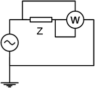

  

  Active power measurement in mono-phase circuits

• (ii) Active power measurement in three-phase circuits is quite similar regardless of load configuration as far as procedure [30]. This consists in connecting a wattmeter in the circuit with the current coil in series with the load and with the voltage coil in parallel with the load. The three-phase circuits have some particularities due to load configurations.

If the load has a neutral line, such as star connected loads, then the power can be measured by using three wattmeters. The voltage coils of the wattmeters are connected between each phase and the neutral point of the load and voltage source [4]. The current coils are connected in series with the load on each phase, as displayed in Fig. 1.19.

Fig. 1.19

Active power measurement in three-phase circuits with neutral line load

If the load does not have an accessible neutral point or is delta connected, in order to measure the power using three wattmeters, these are connected such as to construct an artificial neutral point for them. This situation is indicated in Fig. 1.20. Thus the active power absorbed by the load can be expressed by

Fig. 1.20

Power measurement in three-phase circuits without neutral line load

$$ P = P_{1} + P_{2} + P_{3} $$

(1.28)

If a neutral point is created, it is preferred that it has the same potential as one of the source phase as indicated in Fig. 1.21. In this situation the indication of the third wattmeter would be zero as its voltage coil would be connected at the same potential. Because of this, it is eliminated from the circuit as not being useful. The measured active power is the sum of the indications of each wattmeter, expressed as

Fig. 1.21

Power measurement in three-phase circuits without neutral line load using two wattmeters

$$ P = P_{1} + P_{2} $$

(1.29)

A different situation is the case of balanced loads and symmetrical voltages on each source phase. In this case it is enough to use one wattmeter as indicated in Fig. 1.22. In this situation, the total power is determined by multiplying the indication of the wattmeter by three, as in expressed in Eq. (1.30)

Fig. 1.22

Power measurement for balanced load and symmetrical source voltage with natural neutral point

$$ P = 3 \cdot P_{1} $$

(1.30)

The situation presented in Fig. 1.22 is valid if the load has an accessible neutral point. In case that the load does not have an accessible neutral point, or is delta connected, then it is created an artificial neutral point by using two additional resistors as indicated in Fig. 1.23. The values of the additional resistors R ₁ and R ₂ are equal to the value of the resistance of the voltage circuit of the wattmeter.

Fig. 1.23

Power measurement for balanced load and symmetrical source voltage with an artificial neutral point

5 State of the Art: Standards for Power Systems Parameters

Electrical energy needed to power industrial or household electric consumers, as all the products, should satisfy same quality demands. These demands, like good PQ ensure the electrical equipment is to operate without errors and this is a responsively of the supplier [17, 31].

On the other hand, an important part of the equipment in use today, in particular electronic and computer devices generates distortion of the voltage supply in the installation, because of its non-linear characteristics, i.e. it draws a non-sinusoidal current with a sinusoidal supply voltage. In this case the PQ is a responsively of the electricity user.

In consequence, maintaining satisfactory PQ is a joint responsibility for the supplier and the electricity user.

Standard IEC 60038 distinguishes “two different voltages in electrical networks and installations” [32]:

• supply voltage, which “is the line-to-line or line-to-neutral voltage at the point of common coupling (PCC), i.e. main supplying point of installation”;

• utility voltage, which “is the line-to-line or line-to-neutral voltage at the plug or terminal of the electrical device”.

The main document dealing with demands concerning the supplier’s side is standard EN 50160 [33] which characterize voltage parameters of electrical energy in public distribution systems.

According with Standard EN 50160, “the main voltage characteristics of public distribution systems are”:

Supply voltage—“the root mean square (rms) value of the voltage at a given moment at the PCC, measured over a given time interval”.

Nominal voltage of the system (U _n )—“the voltage by which a system is designated or identified and to which certain operating characteristics are referred”.

Declared supply voltage (U _c )—“is normally the nominal voltage U_n of the system. If, by agreement between the supplier and the user, a voltage different from the nominal voltage is applied to the terminal, then this voltage is the declared supply voltage U _c ”.

Normal operating condition—“the condition of meeting load demand, system switching and clearing faults by automatic system protection in the absence of exceptional conditions due to external influences or major events”.

Voltage variation—“is an increase or decrease of voltage, due to variation of the total load of the distribution system or a part of it”.

Flicker—“impression of unsteadiness of visual sensation induced by a light stimulus, the luminance or spectral distribution of which fluctuates with time”.

Flicker severity—“intensity of flicker annoyance defined by the UIE-IEC flicker measuring method and evaluated by the following signals”:

• Short term severity (P _st ) “measured over a period of ten minutes”;

• Long term severity (P _lt ) “calculated from a sequence of 12 P _st —values over a two-hour interval, according to the following expression”:

$$ P_{lt} = \sqrt[3]{{\sum\limits_{i = 1}^{12} {\frac{{P_{sti}^{3} }}{12}} }} $$

(1.31)

Supply voltage dip—“a sudden reduction of the supply voltage to a value between 90 and 1% of the declared voltage U _c , followed by a voltage recovery after a short period of time”. Conventionally, the duration of a voltage dip is between “10 ms and 1 min”. The depth of a voltage dip is defined as the “difference between the minimum rms voltage during the voltage dip and the declared voltage”.

Supply interruption—is a condition in which “the voltage at the supply terminals is lower than 1% of the declared voltage U _c ”. A supply interruption is classified as:

• “prearranged in order to allow the execution of scheduled works on the distribution system, when consumers are informed in advance”;

• “accidental, caused by permanent (a long interruption) or transient (a short interruption) faults, mostly related to external events, equipment failures or interference”.

Temporary power frequency over-voltages—“have relatively long duration, usually of a few power frequency periods”, and originate mainly from switching operations or faults, e.g. sudden load reduction, or disconnection of short circuits.

Transient over-voltages—“are oscillatory or non-oscillatory, highly damped, short over-voltages with a duration of a few milliseconds or less, originating from lightning or some switching operations”, e.g. at switch-off of an inductive current.

Harmonic voltage—“a sinusoidal voltage with a frequency equal to an integer multiple of the fundamental frequency of the supply voltage”. Harmonic voltages can be evaluated:

• “individually by their relative amplitude U _h related to the fundamental voltage U ₁”, where h is the order of the harmonic;

• “globally, usually by the total harmonic distortion factor THD _u ”, calculated using the following expression:

$$ THD_{u} = \sqrt[{}]{{{{\sum\limits_{h = 2}^{40} {(U_{h}^{{}} )^{2} } } \mathord{\left/ {\vphantom {{\sum\limits_{h = 2}^{40} {(U_{h}^{{}} )^{2} } } {U_{1} }}} \right. \kern-0pt} {U_{1} }}}} $$

(1.32)

Inter-harmonic voltage—“is a sinusoidal voltage with frequency between the harmonics”, i.e. the frequency is not an integer multiple of the fundamental.

Voltage unbalance—“is a condition where rms value of the phase voltages or the phase angles between consecutive phases in a three-phase system is not equal”.

Standard EN 50160 gives the main voltage parameters and their permissible deviation ranges at the customer’s PCC in public low voltage (LV) and medium voltage (MV) electricity distribution systems, under normal operating conditions (Fig. 1.24). In this circumstances, LV signify that the phase to phase nominal rms voltage does not exceed 1000 V and MV signify that the phase-to-phase nominal rms value is between 1 and 35 kV.

Fig. 1.24

Exemplification of a voltage dip and a short supply interruption, classified according to EN 50160; U _n —nominal voltage of the supply system (rms), U _A —amplitude of the supply voltage, U (rms)—the actual rms value of the supply voltage [3]

The comparison of the EN 50160 requirements with those of the EMC standards EN 61000, listed in Table 1.2 show significant differences in various parameters [33,34,35].

Table 1.2 Comparison of supply voltage requirements according to EN 50160 and the EMC standards EN 61000

Harmonic emissions are subject to various standards and regulations [36, 37]:

• “Compatibility standards for distribution networks”;

• “Emissions standards applying to the equipment causing harmonics”;

• “Recommendations issued by utilities and applicable to installations”.

Currently, a triple system of standards and regulations is in force based on the documents listed below.

“Standards governing compatibility between distribution networks and products” determine the necessary compatibility between distribution networks and products:

• The harmonics caused by a device must not disturb the distribution network beyond certain limits;

• Each device must be capable of operating normally in the presence of disturbances up to specific levels;

• Standard IEC 61000-2-2 is applicable for public low-voltage power supply systems;

• Standard IEC 61000-2-4 is applicable for LV and MV industrial installations.

“Standards governing the quality of distribution networks” contain:

• Standard EN 50160 stipulates the characteristics of electricity supplied by public distribution networks;

• Standard IEEE 519 presents a joint approach between utilities and customers to limit the impact of non-linear loads. What is more, utilities encourage preventive action in view of reducing the deterioration of PQ, temperature rise and the reduction of power factor . They will be increasingly inclined to charge customers for major sources of harmonics.

“Standards governing equipment” contain

• Standard IEC 61000-3-2 for low-voltage equipment with rated current under 16 A;

• Standard IEC 61000-3-12 for low-voltage equipment with rated current higher than 16 A and lower than 75 A.

Maximum permissible harmonic levels

An estimation of typical harmonic contents often encountered in electrical distribution networks and the levels that should not be exceeded is presents in Table 1.3.

Table 1.3 Maximum admissible harmonic voltages and distortion (%), h—order of harmonic [36, 37]

Example 1.3

For an assessment of supply voltage, three-phase network, 240 V/400 V are presented the measurement values which was done with PowerQ Plus MI 2392, a portable multifunction instrument for measurement and analysis of three-phase power systems shown in Fig. 1.25. The basic measurement time interval for: voltage, current, harmonics is a 10-cycle time interval. The 10-cycle measurement is resynchronized on each interval tick according to the IEC 61000-4-30 Class B [38, 39]. Measurement methods are based on the digital sampling of the input signals, synchronized to the fundamental frequency. Each input (3 voltages and 3 currents) is simultaneously sampled 1024 times in 10 cycles (Fig. 1.26).

Fig. 1.25

a Power Q-meter, b Measurement stand

Fig. 1.26

Wiring diagram for U, I, f measurements

The supply voltage, which is the line-to-line or line-to-neutral voltage at the PCC [38] i.e. main supplying point of installation. The measured values of supply voltage parameters without and with load (a three-phase asynchronous motor) are presented in Tables 1.4 and 1.5, respectively.

Table 1.4 The parameters values of supply voltage—without load

Table 1.5 The parameters values of supply voltage—with load three-phase asynchronous electric motor 240 V/400 V, 6.6A/3.8 A, 1.5 kW, 1405 rpm, 50 Hz

In concordance with the measured values presented in Tables 1.4 1.5, then:

• voltage magnitude variations: ±10%, means range [216−264 V]/[360–440 V];

• harmonic voltage: 6%-5th, 5%-7th, 3.5%-11th, 3%-13th, THD _u <8%;

• frequency mean value of fundamental measured over 10 s, ±1% (49.5–50.5 Hz).

Thus the electric parameters of public distribution systems, in PCC and the utility voltage satisfy the requirements of standards set.

6 Importance of Reactive Power

Reactive energy and reactive power represent basic signals which are present in all alternating voltage installations, due to their nature and specificity, although they do not produce directly useful effects (light, heat, mechanical work etc.). Most of the time, the realization of useful effects is not possible without reactive energy consumption, taking into account the magnetization processes that take place in motor drives iron cores and in electrical transformers. Also, the leakage fluxes corresponding to the electric lines and to the coils determine reactive power consumption . The resistors, used as electrical energy receivers, consume only active energy, but its transfer through the installations placed upstream reactive determines energy and reactive power losses.

In general, one can say that, in nowadays electrical systems, the active energy and active power management take place only in the presence and with a big consumption of reactive energy and reactive power . From here it results also the concern that, the problems corresponding to producing and management of reactive power and reactive energy to be examined simultaneously with those related to active power and under higher efficiency taking into account their corresponding specificity. At the same time, one should notice also the signal that expresses the correlation between the two powers and energies categories that is the power factor PF, as a main signal for guiding the corresponding problems analysis.

As a general aspect for reactive power and reactive energy management in electrical installations, one considers as necessary, to underline the essential difference between the process required to produce active power and active energy that takes place, in principal, in electric power plants, belonging to the energetic system and the one corresponding to producing reactive energy and reactive power. This is due to that active energy production implies primary energy consumption, which is not the case of the reactive energy, excepting the case for covering some active energy losses, reduced as signal.

The necessity to have a reactive power flow control arises from the fact that, practically, in each station, for solving sinusoidal states, the adopted solution is that of using capacitor banks. These are installed, usually, on LV mains power supply of the transformer power, where are connected the consumers from all or from a part of the enterprise. The purpose, with priority, is to obtain an overall power factor, at least equal to the neutral value (imposed by the electrical energy provider contract), in the point used for measuring the active and reactive energy consumption of the electrical installations placed downstream, avoiding the overcompensation situations. In general, for the energy provided to the consumers, the values obtained for the overall power are in 0.93 … 0.97 range.

Many factories use also automatic multi-step power factor correction systems (MSPFC), to maintain constant value for the power factor. This is the situation for long-term functioning in industrial installations, on the occasion of the current jobs. One can affirm this solution contributes to a rational management of the reactive energy and reactive power, representing a priority in the electrical energy sector.

The analysis of this aspect is done, in general, at the enterprises level, because the electrical energy consumers from this one, and especially the operation, with very large nominal power range, sometimes due to over-sizes, as well as the corresponding low-loaded functioning, have the biggest weight from the general reactive power consumption , sometimes up to 60–70%.

The transformers from the electroenergetical system take around 20% out from the reactive power , the rest of the consumption belonging to the other installations.

The solution of placing a capacitor bank in the transformer power substation under the name of global compensation, presents advantage only for upstream installations, exterior to the enterprise, respectively for generating, transport and distribution installations. Using this type of compensation, the advantage represented by reactive and active power and energy losses, does not appear also for enterprise’s installations. From this point of view the installations from the enterprise do not benefit from the advantage given by reactive power local production.

Taking into account the importance of the contribution, given by reactive power compensation measures, also to the losses reduction in distribution installation inside the enterprise, is indicated that, for on-going processes, to examine also the possibilities to de-centralize the banks in proper installations, that is to use with more economical compensation types, respectively, the individual or by sector consumers.

It is necessary to notice that, a special importance for consumers and electroenergetical system reactive power management, the apparition of new types of receivers, with non-linear electrical characteristics critically influence the reactive power management. The presence of the harmonic state, in many cases, determines practically the total revision of the compensation used currently, by exclusively installing the capacitor banks. This fact is determined by the reciprocal influence of these two aspects, the reactive power compensation and the harmonic, implying the application of a unique measure, respectively that of using filters that include also the existing capacitor banks.

Due to the complexity of the two problems and especially to the necessity and of the urgency of solving a phenomena assembly, one will examine, as follows, the most important theoretical and technical-economical specific aspects, that can be used to establish the on-going processes. In all cases, one should analyze, together, the two problems, taking into account that practically all modern electrical energy consumers present a nonlinear characteristic.

6.1 Reactive Power Flow Effects Evaluation

Electric devices are designed at a certain apparent power S that is proportional to the product between the rms values corresponding to the voltage U and to the current I. The power flow in the electroenergetical system is accompanied, function of the electric energy consumer structure, by the active power flow P, reactive power flow Q and distorted power flow D. The only useful one is the active power flow and its corresponding share from the apparent power necessary is computed using the power factor  PF defined as [40]:

$$ PF = \frac{P}{S} = \frac{P}{{\sqrt {P^{2} + Q^{2} + D^{2} } }} $$

(1.33)

The weights corresponding to the reactive and distorted powers are estimated using the reactive factor ρ and the distorted factor τ for the permanent harmonic state, according to the relationships

$$ \rho = \frac{Q}{P} = \tan \varphi ;\quad \tau = \frac{D}{{\sqrt {P^{2} + Q^{2} } }} = \tan \psi \, $$

(1.34)

where the phasors P, Q, D form a three-orthogonal reference system, and the phase-shifts φ and ψ have the significance given in Fig. 1.27.

Fig. 1.27

Significance of phase-shifts φ and ψ

So, one obtains a new expression for the power factor $k = \cos \phi \cdot \,\cos \psi$. If one considers a sinusoidal permanent single-phase circuit, then: $D = 0{ (}\psi = 0 )$ and $k = \cos \varphi$ so the power factor is numerically equal to the cosine of phase-shift angle between the voltage and the current.

For three-phase equilibrium circuits, linear and sinusoidal voltage powered, the power factor has exactly the same mathematical expression and significance as for single-phase circuit case. If the electric circuits are slightly asymmetrical, then the voltage-current phase-shifts are different from a phase to another $\varphi_{1} \ne \varphi_{2} \ne \varphi_{3}$ and the power factor will be:

$$ PF = \frac{{P_{1} + P_{2} + P_{3} }}{{\sqrt {(P_{1} + P_{2} + P_{3} )^{2} + (Q_{1} + Q_{2} + Q_{3} )^{2} } }} $$

(1.35)

where P _j and Q _j are the active, respectively the reactive powers corresponding to each one of the phases (j = 1, 2, 3).

The relationships above define the instantaneous power factor that corresponds to a certain moment form the consumer’s installation functioning. Because the load presents fluctuations, the current legislation recommends the determination of the weighted overall power factor based on the active and reactive energy consumption E _a , E _r from a certain period, in the hypothesis that the receivers behave as a linear three-phase load, in equilibrium, working in sinusoidal permanent state:

$$ \cos \varphi = \frac{{E_{a} }}{{\sqrt {E_{a}^{2} + E_{r}^{2} } }} $$

(1.36)

Related to the weighted overall power factor , this can be neutral when is being determined without taking into consideration the reactive power compensation installations, and general, when one takes into account the powers provided by these installations. The value of the general weighted overall power factor from which the reactive energy power consumption is no longer charged, is called neutral power factor and for the national energetic system is $\cos_{n}^{*} = 0,92$.

For electrical installations inside the consumer: the power factor decreasing causes, the effects of a reduced power factor, means and methods for power factor mitigation, a technical-economical computation for placing the reactive power sources etc.

The irrational and big reactive power consumption , that generates a reduced power factor , presents a series of disadvantages for the electric installation, among which we mention [25]: the increase of active power losses in the passive elements of the installation, the increase of voltages’ losses, installation’ oversize and the its electric energy diminished transfer capacity.

6.2 Harmonic State Indicator—Specific PQ Parameters

Electrical installations that contain non-linear consumers absorb non-sinusoidal electric current even in the theoretical case of a perfect sinusoidal voltage supply. The non-sinusoidal electric current flows through the impedances corresponding to these electrical installations determine non-sinusoidal voltage drops that, superposed over the initial sinusoidal voltage signals, determine their distortion (shown in Fig. 1.28). This determines a supplementary solicitation of the electrical installations.

Fig. 1.28

Fourier series decomposition of a periodic distorted voltage signal

According to Fourier theory [3, 7] the periodic distorted signals can be decomposed in sinusoidal components whose frequencies are integer multiple of the frequency corresponding to the analyzed signal period. The sinusoidal signal with reference frequency (that corresponds to the analyzed period signal) is called fundamental signal, and the sinusoidal signals with frequency integer multiple of the fundamental frequency are called harmonics.

$$ \begin{aligned} & u = U_{0} + \sum\limits_{k = 1}^{\infty } {\sqrt 2 U_{k} \sin (k\omega_{1} t + \alpha_{k} );} \\ & i = I_{0} + \sum\limits_{k = 1}^{\infty } {\sqrt 2 I_{k} \sin (k\omega_{1} t + \beta_{k} )} \\ \end{aligned} $$

(1.37)

where: U ₀ and I ₀ represents the DC components of the input voltage and current, U _k and I _k are the rms values of harmonic voltages, respectively of the harmonic currents, ω ₁ pulsation corresponding to the fundamental frequency, α _k , β _k —phase-shifts corresponding to the harmonic voltages signals, respectively to harmonic currents signals with respect to a reference axis.

To define the main indicators of harmonic state, we consider, as a reference periodic signal, the electric wave shape through the load i(t) developed in Fourier series. The following definitions are valid for any periodic signal [41, 42].

• Harmonic level—is defined as the ratio between the rms value of the harmonic of rank k and the rms value of the fundamental harmonic (rank 1):

$$ \gamma_{k} [\% ] = \frac{{I_{k} }}{{I_{1} }} \cdot 100[\% ] $$

(1.38)

This factor is an important indicator for evaluating the distortion level, its maximum admitted values is being indicated in the voltage or current signal.

• DC−component of the signal is defined as the integral on a variation signal period:

$$ \left\langle I \right\rangle = DC = \frac{1}{T}\int\limits_{{t_{0} + T}}^{T} {i(t)dt} = I_{0} $$

(1.39)

The mean value of a signal different from zero indicates the presence of a DC component in its spectrum.

• Crest factor−CF—defined as the ratio between the maximum value (amplitude i _M of the periodic non-sinusoidal signal) and its rms value I _RMS :

$$ k_{v} = CF_{i} = \frac{{i_{M} }}{{I_{RMS} }} $$

(1.40)

• for a pure sine wave, k _v  = 1.41;

• for periodic “shaped-top” distorted waveform signal k _v  > 1.41;

• for a periodic “flat-top” distorted waveform signal k _v  < 1.41.

The voltage signals characterized by a crest factor $k_{vi} > \sqrt 2$ can present in time dangerous thermal solicitations.

• Form Factor—is the ratio between the rms value of the signal and the mean value corresponding to half a period I _med1/2:

$$ k_{f} = \frac{I}{{I_{med1/2} }} = k_{f} = \frac{{I_{RMS} }}{{\frac{1}{T}\int\limits_{{t_{0} }}^{{t_{0} + T}} {\left| {i(t)} \right|dt} }} $$

(1.41)

For the signals met in electrical installations the form factor can take the values:

• for a sinusoidal signal, k _f  = 1.11;

• for a periodic signal shaper than a sinusoid k _f  > 1.11;

• for a sinusoid flatter than a periodic signal k _f  < 1.11.

• Root Mean Square—rms Value:

$$ I_{RMS} = \sqrt {\frac{1}{T} \cdot \int\limits_{0}^{T} {i^{2} \cdot dt} } \, {\text{or}}\,I_{RMS} = \sqrt {I_{0}^{2} + I_{1}^{2} + I_{2}^{2} + \ldots } = \sqrt {\sum\limits_{k = 0}^{n} {I_{k}^{2} } } $$

(1.42)

Remarks:

• For signals containing harmonics one uses the terminology True rms Value. To compute it, one should take into also the high-order harmonics (usual up to 50!).

• Not all measuring equipment can correctly measure the rms value of a non-sinusoidal signal (True rms Value), many of them displaying only the rms value corresponding to the fundamental (first harmonic)!

• Residual component (I _d )—is computed as the rms value of the harmonics corresponding to the analyzed signal:

$$ I_{d} = \sqrt {I_{RMS}^{2} - I_{1}^{2} } \cong \sqrt {I_{0}^{2} + I_{2}^{2} + I_{3}^{2} + \ldots } $$

(1.43)

The distortion residue is a measure if the thermal effect determined by the distorted signal harmonic components.

• Total Harmonic Distortion −THD—is the ratio between the distortion residue of the signal and the fundamental rms value:

$$ THD_{i} = \frac{{I_{d} }}{{I_{1} }} = \frac{{\sqrt {I_{RMS}^{2} - I_{1}^{2} } }}{{I_{1} }} = \frac{{\sqrt {I_{2}^{2} + I_{3}^{2} + I_{3}^{2} + \cdots } }}{{I_{1} }} = \frac{{\sqrt {\sum\limits_{k = 2}^{n} {I_{k}^{2} } } }}{{I_{1} }} \cdot 100\,[\% ] $$

(1.44)

The THD is one of the indicators used to evaluate the distortion level, the maximum admitted values in the electrical network nodes being tabled [43].

• Distortion Factor−DF—is defined as the ratio between the distorted residue of the signal and the rms value of the signal:

$$ DF_{i} = \frac{{I_{d} }}{{I_{RMS} }} = \frac{{\sqrt {I_{RMS}^{2} - I_{1}^{2} } }}{{I_{RMS} }} = \frac{{\sqrt {I_{2}^{2} + I_{3}^{2} + I_{3}^{2} + \cdots } }}{{I_{RMS} }} = \frac{{\sqrt {\sum\limits_{k = 2}^{n} {I_{k}^{2} } } }}{{I_{RMS} }} \cdot 100\,[\% ] $$

(1.45)

The DF is much closed as value to THD and it is used also as a principal indicator for appreciating the distortion level.

Remark:

• In literature [44, 45], THD is also denoted by THD-F (distortion related to the fundamental) and DF can be found denoted by THD-R (distortion related to the rms value)

• One can easily prove the relationship: $\frac{{I_{1} }}{{I_{rms} }} = \frac{1}{{\sqrt {1 + THDi^{2} } }}$

• The derating factor KF of the transformer’s apparent power—is defined (only for electric current) as follows:

$$ KF = \frac{{\sum\limits_{k = 1}^{n} {\left( {kI_{k} } \right)^{2} } }}{{\sum\limits_{k = 1}^{n} {I_{k}^{2} } }} $$

(1.46)

where I _k is the rms value of the harmonic of rank k of the electric current that flows through the transformer’s windings. KF (defined only for the current) allows an evaluation of the supplementary heating of the transformers circulated by distorted currents that imply derating its installed power [46, 47].

In order to evaluate the energetic indicators of harmonic state, one defines the following types of powers:

• Single-phase active power P (active power) for harmonic state is:

$$ P = \frac{1}{m \cdot T} \cdot \int\limits_{\tau }^{\tau + m \cdot T} {pdt = } \frac{1}{mT}\int\limits_{\tau }^{\tau + m \cdot T} {uidt} = \sum\limits_{h = 1}^{\infty } {U_{k} I_{m} \cos \varphi_{k} } \;\left[ {\text{W}} \right] $$

(1.47)

where φ _k = α _k  − β _k is the phase-shift between the signals corresponding to the voltage and to the current, in the plan of harmonic of rank k.

• Active energy W _a in harmonic state is:

$$ W_{a} = \int\limits_{\tau }^{\tau + t} {P \cdot dt} \,\left[ {\text{Ws}} \right] $$

(1.48)

• Single-phase reactive power Q (reactive power) is given by the expression:

$$ Q = \sum\limits_{k = 1}^{\infty } {U_{k} I_{k} \sin \varphi_{k} } \;\left[ {\text{VAr}} \right] $$

(1.49)

• Single-phase reactive energy W _r in harmonic state is:

$$ W_{r} = \int\limits_{\tau }^{\tau + t} {Q \cdot dt} \,\left[ {\text{VArs}} \right] $$

(1.50)

• Single-phase apparent power S (apparent power) is defined by the expression:

$$ \begin{aligned} S & = U_{RMS} I_{RMS} = \sqrt {U_{0}^{2} + U_{1}^{2} + U_{2}^{2} + \ldots } \cdot \sqrt {I_{0}^{2} + I_{1}^{2} + I_{2}^{2} + \ldots } \\ & = \sqrt {\sum\limits_{k = 0}^{n} {U_{k}^{2} } \cdot } \sqrt {\sum\limits_{k = 0}^{n} {I_{k}^{2} } } \\ \end{aligned} $$

(1.51)

• Single-phase apparent energy W is defined by:

$$ W = \int\limits_{\tau }^{\tau + t} {S \cdot dt} \,\left[ {\text{VAs}} \right] $$

(1.52)

• Distorted power—is defined as a complement of active and reactive power related to the apparent power:

$$ D = \sqrt {S^{2} - P^{2} - Q^{2} } \quad \left[ {\text{VAd}} \right] $$

(1.53)

Remark:

• Most modern measuring equipment designed for measuring electric energy and electric power can measure instantly each of the 4 defined powers (energies).

• Power Factor −PF—is defined as the ratio between the active power P and the total apparent power S:

$$ \lambda = PF = \frac{P}{S} = \frac{{\sum\limits_{k = 1}^{\infty } {U_{k} I_{k} \cos \varphi_{k} } }}{{U_{RMS} I_{RMS} }} $$

(1.54)

• Displacement Power Factor−DPF—is defined as the ratio between the active power P ₁ and the apparent power S ₁, corresponding to the fundamental harmonic (k = 1):

$$ \lambda_{1} = DPF = \frac{{P_{1} }}{{S_{1} }} = \frac{{U_{1} I_{1} \cos \varphi_{1} }}{{U_{1} I_{1} }} = \cos \varphi_{1} $$

(1.55)

Remarks:

• The two definitions for PF and DPF leads to different values displayed separately by modern measuring equipment. Moreover, the value of the angle φ ₁ and its tangent tan φ ₁ are also displayed.

• The equality $\lambda = \frac{P}{S} = \cos \varphi \;(PF = DPF)$ is valid only for a single-phase circuit and only in a pure sinusoidal state (ideal case), so the interpretation of the power factor function of voltage-current phase-shift should be avoided!

• If, it’s necessary, the dimensioning of a capacitor bank for reactive power compensation can be done only based on power factor cosφ ₁ = DPF and not on PF!

• One can easily prove the relationship: $PF = \frac{{\cos \varphi_{1} }}{{\sqrt {1 + THDi^{2} } }} = \frac{DPF}{{\sqrt {1 + THDi^{2} } }}$ (valid in the case of negligible voltage distortion THD _u  < 5%).

Most of the above mentioned parameters are nowadays commonly indicated by high accuracy measurement devices such PQ analyzers. They are able to perform a complete Fourier analysis for the three-phase current and voltage signals up to the 50 harmonic. Figure 1.29 illustrates these parameters measured with a Chauvin Arnoux 8335 device for a low-voltage industrial load.

Fig. 1.29

Current signals, harmonics and various PQ parameters measured for a low-voltage industrial load

General solutions for reducing the reactive power consumption are [48,49,50]:

• adopting, if possible, some technological processes , aggregates and technological and functioning schemes, characterized by a high power factor ;

• judicious choice of the type and powers for the electric motor drives, for the transformers, avoiding over-sizing; introducing the synchronous motor instead of the asynchronous one will be justified from economical point of view considering the asynchronous motor individually compensated with derivation capacitors.

The principal means used especially in existing installations are the following:

• power transformers running in parallel, following the minimum reactive losses graph, when the exploitation conditions allow it;

• exploitation of synchronous motors at the maximum limit of producing reactive power;

• limiting the unloaded running of asynchronous motors, of special transformers, if the technological process allows it;

• using Y-Δ switches for low-voltage asynchronous motors, systematically loaded under 40% from its nominal load, for a long-term functioning in Y connection;

• replacing asynchronous motors and of the over-sized transformers, based on technical-economic analysis using the updated total spending method.

The main specialized reactive power sources are synchronous compensators and derivation capacitors.

Reactive power control has a significant role in role in supporting the power transmission systems .

Reactive power is required to deliver active power through transmission lines at a certain voltage level. Motors, transformers and other power loads, intrinsically require reactive power in order to maintain their functionality. Either the lake or the excess of reactive power may lead to numerous PQ disturbances, which adversely affect both the loads and the supply network [16].

References

J.C. Maxwell, A Treatise on Electricity and Magnetism, 3rd ed. vol. 1 and 2, New York, Dover Publication, 1954.
V. Bellevitch, Classical Network Theory, Holden-Day, 1968.
L.O. Chua, Nonlinear Network Theory, New York, McGraw Hill, 1969.
P. Penfield Jr, R. Spence, S. Duinker, Tellegen’s Theorem and Electrical Networks, Research monograph no. 58, Massachusetts, M.I.T. Press, 1970.
R.W. Newcomb, Linear Multiport Synthesis, New York, McGraw-Hill, 1966.
M. Preda, P. Cristea, Fundamentals of Electrotechnics (in Romanian: Bazele Electrotehnicii), vol. 2, Bucharest, ed. Didactica si Pedagogica, 1980.
C.A. Desoer, E.S. Kuh, Basic Circuit Theory, New York, Mc Graw-Hill, 1969.
J.C. Willems, Dissipative and Dynamical Systems, Eur. J. Contr., vol. 13, pp. 134–151, 2007.
M. Vasiliu, I.F. Hantila, Electromagnetics, Bucharest, ed. Electra, 1st ed., 2006.
C.I. Mocanu, Electromagnetic Field Theory (in Romanian: Teoria Campului Electromagnetic, Bucharest, ed. Didactica si Pedagogica, 1st ed., 1981.
C.I. Mocanu, Electric Circuits Theory (in Romanian: Teoria circuitelor electrice) Bucharest, ed. Didactica si Pedagogica, 1st ed., 1979.
H. Andrei, Modern Electrical Engineering (in Romanian: Inginerie Electrica Moderna), vol. 1, ed. Bibliotheca, Targoviste, 2010.
J. Arrillage, N. Watson, S. Chen, Power System Quality Assessment, John Wiley & Sons, New York, 2001.
L.F. Beites, J.G. Mayordomo, A. Hernandes, R. Asensi, Harmonics, Inter Harmonic, Unbalances of Arc Furnaces: A New Frequency Domain Approach, IEEE Transactions on Power Delivery, 16(4), 2001, 661–668.
C. Cepisca, H. Andrei, S. Ganatsios, S.D. Grigorescu, Power Quality and Experimental Determinations of Electrical Arc Furnaces, Proc. 14th IEEE Mediterranean Electrotechnical Conference, MELECON, vol. 1 and 2, pp. 546–551, Ajaccio France, May 5–7, 2008.
A.E. Emmanuel, On the Assessment of Harmonic Pollution, IEEE Transaction on Power Delivery, vol. 10(3), 1995, 1693–1698.
A. Eberhard, Power Quality, InTech, Vienna, 2011.
A.E. Emmanuel, Apparent Power Definition for Three-Phase systems, IEEE Transactions on Power Delivery, 14 (3), 1999, 762–772.
J. Zhu, Optimization of Power System Operation, Willey & Sons, 2009.
P.S. Filipski, Y. Baghzouz, M.D. Cox, Discussion of Power Definitions Contained in the IEEE Dictionary, IEEE Transaction on Power Delivery, vol. 9(3), 1994, 1237–1244.
E.F. Fuchs, M.A.S. Masoum, Power Quality in Power Systems and Electrical Machines, Elsevier Academic Press, Amsterdam, 2006.
R. Hurst, Power Quality and Grounding Handbook, The Electricity Forum, Toronto, Canada, 1994.
V. Katic, Network Harmonic Pollution - A Review and Discussion of International and National Standards and Recommendations, Proc. of Power Electronic Congress - CIEP, pp. 145–151, Paris, France, October 24–26, 1994.
T.S. Key, J.S. Lai, IEEE and International Harmonic Standard Impact on Power Electronic Equipment Design, Proc. of International Conference Industrial Electronics, Control and Instrumentation - IECON, pp. 430–436, London, England, May, 25–27, 1997.
C. Sankaran, Power Quality, CRC Press, London, 2008.
P. Arpaia, Power Measurement, CRC Press LLC, 2000.
B. Gatheridge, How to Measure Electrical Power, EDN Network, 2012.
S. Humphrey, H. Papadopoulos, B. Linke, S. Maiyya, A. Vijayaraghavan, R. Schmitt, Power Measurement for Sustainable High-Performance Manufacturing Processes, Procedia CIRP, vol. 14, pp. 466–471, 2014.
M.A. Lombardi, Fundamentals of Time and Frequency, http://tf.nist.gov/general/pdf/ 1498.pdf, Accessed July 2015.
Oscilloscope, https://en.wikipedia.org/wiki/Oscilloscope.
H. Markiewicz, A. Klajn, Power Quality Application Guide, Wroclaw University of Technology, July 2004.
IEC 6038 - International Electrotechnical Commission Standard Voltages, 1999.
EN 50160 - European Norm Voltage Characteristics of Electricity Supplied by Public Distribution Systems, 1999.
IEC 61000-4-7, International Electrotechnical Commission.
IEC 61000-4-15, International Electrotechnical Commission.
F.C. De La Rosa, Harmonics and Power Systems, New York, Taylor & Francis, 2006.
Electrical Installation Guide, Schneider Electric, 2015.
Technische Anschlussbedingungen (Technical requirements of connection), VDEW.
Rozporzadzenie Ministra Gospodarki z dnia 25 wrzesnia 2000, w sprawie szczególowych warunków przylaczania podmiotów do sieci elektroenergetycznych, obrotu energia elektryczna, swiadczenia uslug przesylowych, ruchusieciowego i eksploatacji sieci oraz standardów jakosciowych obslugi odbiorców. Dziennik Ustaw Nr 85, poz. 957 (Rules of detailed conditions of connection of consumers to the electrical power network and quality requirements in Poland).
A.E. Emanuel, Power Definitions and the Physical Mechanism of Power Flow, John Wiley & Sons, 2011.
A. Baggini, Handbook of Power Quality, John Wiley & Sons, 2008.
IEEE 100-1996, The IEEE Standard Dictionary of Electrical and Electronics Terms, 6th Edition, 1996.
IEEE-WG, IEEE Working Group on Nonsinusoidal Situations, Practical Definitions for Powers in Systems with Nonsinusoidal Waveforms and Unbalanced Loads, IEEE Transactions on Power Delivery, vol. II, no. 1, 1996, 79–101.
R.C. Dugan, M.F. McGranaghan, S. Santoso, H.W. Beaty, Electrical Power Systems Quality, McGraw Hill Professional, 2012.
A. Kusko, M. Thomson, Power Quality in Electrical Systems, McGraw Hill Professional, 2007.
IEC 61000-4-30, Testing and Measurement Techniques-Power Quality Measurement Method, 1999.
IEEE Recommended Practice for Monitoring Electric Power Quality, IEEE 1159, 1995.
Romanian Norm for Limitation of Harmonic Pollution and Unbalance in Electrical Networks, PE 143, 2004.
Characteristics of Supplied Voltage in Public Distribution Networks, SREN 50160, October 1998.
Power Quality Application Guide, Voltage Disturbance, Standard EN50160, July 2004.
Author information
Authors and Affiliations
Corresponding author
Editor information
Editors and Affiliations
Rights and permissions
Copyright information
© 2017 Springer International Publishing AG
About this chapter
Cite this chapter
Andrei, H., Andrei, P.C., Constantinescu, L.M., Beloiu, R., Cazacu, E., Stanculescu, M. (2017). Electrical Power Systems. In: Mahdavi Tabatabaei, N., Jafari Aghbolaghi, A., Bizon, N., Blaabjerg, F. (eds) Reactive Power Control in AC Power Systems. Power Systems. Springer, Cham. https://doi.org/10.1007/978-3-319-51118-4_1
Download citation
DOI: https://doi.org/10.1007/978-3-319-51118-4_1
Published:
Publisher Name: Springer, Cham
Print ISBN: 978-3-319-51117-7
Online ISBN: 978-3-319-51118-4
eBook Packages: EnergyEnergy (R0)