
Abstract
We present a novel approach to characterize multiple sclerosis (MS) from brain magnetic resonance imaging (MRI) with geostatistics. Brain MRI provides excellent, exhaustive input data to geostatistical analysis, typically several million voxels per MRI scan. A dataset of 259 spatially normalized binary MS white matter lesion (WML) patterns covering very mild to extremely severe MS cases was subject to directional variography. Using an exponential variogram model function, the observed spatial variability in x,y,z directions can be expressed by geostatistical parameters range and sill which perfectly correlate with WML pattern surface complexity and lesion volume. A scatterplot of ln(range) vs. ln(sill), classified by pattern anisotropy, enables a consistent and clearly arranged presentation of MS-lesion patterns based on their geometry. The geostatistical approach and the graphical representation of results are considered efficient exploratory data analysis tools for longitudinal, cross-sectional, and medication impact studies.
Access provided by CONRICYT-eBooks. Download chapter PDF
Keywords
- Multiple Sclerosis
- Multiple Sclerosis Patient
- White Matter Lesion
- Magnetic Resonance Imaging Data
- Multiple Sclerosis Lesion
These keywords were added by machine and not by the authors. This process is experimental and the keywords may be updated as the learning algorithm improves.
1 Introduction
Multiple sclerosis (MS) is an autoimmune disease of the central nervous system (CNS) that causes inflammatory demyelinating lesions in the brain and in the spine. MS affects over 2.5 million people worldwide and is the primary nontraumatic cause of neurologic disability in young adults, with an associated socioeconomic impact. The individual course of MS is highly variable – while some patients may acquire severe and irreversible disability within a few years, others may follow a mild course with almost no disability even after decades (Compston and Coles 2008).
2 MRI Data
The introduction of magnetic resonance imaging (MRI) for MS diagnosis and monitoring the disease course was a milestone in MS patient’s care (Filippi and Rocca 2011). Recent diagnostic criteria allow setting MS diagnosis on the basis of MRI (Polmann et al. 2011). The hallmark of MS is hyperintense sclerotic lesions within cerebral white matter, as indicated in Fig. 1 which is a T2-weighted (FLAIR) axial slice through an MS patient’s brain.

MRI of MS-affected brain. Arrows indicate bright, hyperintense MS lesions (FLAIR MRI sequence, axial slice at top of ventricle system)
Traditionally, MRI scanners yield stacks of parallel images from which 3D models can be derived; more recent MRI scanners provide voxel models which directly represent the volume of interest. Before single-patient follow-up MRI scans (longitudinal studies) or multiple-patient MRI scans (cross-sectional studies) can be compared, the individual brain scans need to be geometrically matched to a standard brain template like the Montreal Normal Brain (“MNB,” Collins et al. 1998; Penny et al. 2007). This approach compensates for varying head positions in follow-up MRI scans and ensures reference brain geometry when working with group data (Fig. 2).

Geometrical transformation of individual brain geometry (left) to MNB geometry (right). Axial slice of MS-affected brain at top of ventricle level
From MRI data, 3D MS-lesion patterns can be extracted with semiautomatic or automatic lesion extraction software that outputs binary MS-lesion models (Garcia-Lorenzo et al. 2012).
3 The Geostatistical Approach
WML presents rather heterogeneously across patients not only with regard to the number and overall volume but also with regard to spatial pattern, predilection sites, and shape of single lesions. Routine radiological evaluation reports the number of WML, the total lesion load (volume), and the associated changes as from follow-up investigations. Our goal is to describe the spatial structure of a WML pattern in MNB geometry with standard geostatistical parameters (Marschallinger et al. 2014, 2016).
Since the MNB can be considered a Euclidean space which is then dissected into equally sized voxels, the constant extent and support of the MNB enable rapid, grid-based variography (Eq. 1), variogram modeling (Eq. 2), and the sensitive comparison of longitudinal and cross-sectional studies.
For efficient characterization of WML from MRI, we developed the following, fully automatic processing pipeline that builds on a pair of T1 and FLAIR MRI images, acquired on a 3-tesla scanner:
-
1.
From FLAIR and T1 sequences of a single MRI investigation, automatically derive a binary 3D model of the WML pattern in MNB geometry (e.g., Fig. 3 right). Software used is Lesion Segmentation Tool (LST) (Schmidt et al. 2012).
Fig. 3 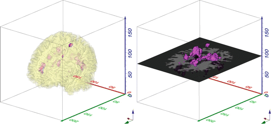
Left: 3D model of white matter of MS-affected brain, normalized to MNB geometry (white matter visualized in translucent style to show some MS lesions for orientation in 3D). Right: associated WML model, white matter striped off, and axial slicing plane at ventricle level indicated for orientation. MNB geometry
-
2.
Compute directional empirical variograms (Eq. 1) in x,y,z directions (dextral-sinistral, caudal-rostral, dorsal-ventral orientations). Variograms are confined to lag distances from 0 to 15 mm, because this area holds the most relevant correlation information and a variogram model can be fitted straightforwardly. Software used is Geostatistical Software Library (GSLIB) (Deutsch and Journel 1997).
-
3.
Fit an exponential variogram model function (Eq. 2) to each directional empirical variogram to yield associated range and sill parameters. These characterize overall surface smoothness, total lesion volume (TLL, total lesion load), and preferred spatial continuity of a white matter lesion (WML) pattern. Software used is R (R development core team 2008).
-
4.
Derive scatterplots of ln(range) vs. ln(sill) to portray WML patterns in a space defined by total pattern surface smoothness vs. total lesion volume. For the current purpose, “surface smoothness” is defined as the ratio of total WML pattern volume/total WML pattern surface. This space, making up the so-called MS-Lesion Pattern Discrimination Plot (LDP), enables a clear presentation of the spatial characteristics of a WML pattern. Scatterplots involving individual x,y,z directions account for anisotropy in WML geometry. Calculating mean center (e.g., De Smith et al. 2007) for a WML from x,y,z directional ln(range) and ln(sill) data, the overall x,y,z geometry of a WML can be expressed. Since all parameters are derived from geometrically standardized data (i.e., MNB geometry), in the course of longitudinal and cross-sectional studies, WML patterns can be immediately related: On the one hand, data can be compared synoptically; on the other hand, they are ready for automatic processing, e.g., for deriving evolution paths in single-patient follow-up from mean center data (Fig. 6).

The LDP conveniently combines class symbols indicating the number of individual lesions (Fig. 4) or standard distance (De Smith et al. 2007) to express overall WML anisotropy. Working through Fig. 4 shows that complex patterns with many lesions or patterns with a “rough”/“complex” surface generally are positioned at the left fringe of the point cloud while patterns with few, big, and “smooth” lesions are placed toward the right border. Patterns around the long axis of the elliptic cloud mediate between rough and smooth extremes.

Combining geostatistical Range ln(a) and geostatistical Sill ln(C) of 259 MS-affected, geometrically normalized brains in the MS-Lesion Pattern Discrimination Plot (LDP). Four WML pattern 3D models and their associated positions in the LDP are indicated. nLesions: number of individual lesion objects per WML pattern, coded by symbols. See text for details (After Marschallinger et al. 2016)
More clinically relevant, the LDP can be used to portray the evolution of WML during single-patient follow-up. Figure 5 shows WML patterns from MRI follow-ups of three patients. Each patient was scanned three times at 6-month intervals, yielding a total observation period of 1.5 years per patient. Patients are arranged in rows, and columns represent MRI investigations (time series advancing from left to right, also indicated by WML colors red-yellow-green). Using the abovementioned processing pipeline, the evolution of the three individual WML patterns can be visualized and quantitatively described by means of the LDP (Fig. 6). In Fig. 5, Patient 1 shows a decrease in MS lesion sizes and concurrent decrease in surface smoothness due to decomposition of big MS lesions into smaller ones; accordingly, in the LDP, the evolution path arrows point to lower volumes and a less smooth overall surface (Fig. 6). About the same is due for Patient 3; the WML pattern of which shows volume loss at the cost of lesion pattern smoothness. This is more pronounced between scans two and three where the biggest lesion continues to decrease but new small lesions show up, yielding approximately constant volume. Patient 2 shows increasing lesion volume at increasing WML pattern surface smoothness caused by confluence of small lesions into bigger ones.

WML evolution in three MS patients, three time steps each chronology from left to right, time interval 6 months each. (See text for details, compare with Fig. 6)

WML pattern evolution paths of three MS patients in the LDP. Arrows indicate evolution direction. Compare Fig. 5 (See text for details)
4 Conclusions
A workflow and processing pipeline has been established that enables the characterization of MS-related white matter lesion (WML) patterns from MRI data by estimation of geostatistical parameters’ range and sill. These are the bases for representing a WML pattern in the MS-Lesion Pattern Discrimination Plot (LDP). The LDP is a versatile framework that combines WML pattern volume, WML pattern surface smoothness, and geometrical anisotropy information in a single, well-arranged plot. Major changes as well as subtle fluctuations in MS-lesion pattern geometry can be visualized straightforwardly. The LDP provides precise insight into the spatial development of WML patterns (i.e., selective growth/shrink in specific directions) without requiring object-based characterization. The LDP is considered an EDA tool that informs on the spatial/spatiotemporal properties of WML patterns in cross-sectional and longitudinal studies and in monitoring medication efficacy.
References
Collins DL, Zijdenbos AP, Kollokian V et al (1998) Design and construction of a realistic digital brain phantom. IEEE Trans Med Imag 17(3):463–468
Compston A, Coles A (2008) Multiple sclerosis. Lancet 372:1502–1517
De Smith M, Goodchild M, Longley PA (2007) Geospatial analysis. Matador, Leicester, 491 pp
Deutsch CV, Journel AG (1997) GSLIB Geostatistical software library and user’s guide. Oxford University Press, 380pp
Filippi M, Rocca MA (2011) MR imaging of multiple sclerosis. Radiology 259(3):659–681
Garcia-Lorenzo D, Francis S, Narayanan S, Arnold DL, Collins L (2012) Review of automatic segmentation methods of multiple sclerosis white matter lesions on conventional magnetic resonance imaging. Med Image Anal 17:1–18
Marschallinger R, Golaszewski S, Kunz A et al (2014) Usability and potential of geostatistics for spatial discrimination of multiple sclerosis lesion patterns. J Neuroimaging 4(3):278–286. doi:10.1111/jon.12000
Marschallinger R, Schmidt P, Hofmann P, Zimmer C, Atkinson P, Sellner J, Trinka E, Mühlau M (2016) A MS-lesion pattern discrimination plot based on geostatistics. Brain Behav 6(3), doi: 10.1002/brb3.430
Penny WD, Friston JK, Ashburner JT, Kiebel SJ, Nichols TE (2007) Statistical parametric mapping: the analysis of functional brain images. Academic Press, London, 625pp
Polmann CH, Reingold SC, Banwell B et al (2011) Diagnostic criteria for multiple sclerosis: 2010 revisions to the McDonald criteria. Ann. Neurology 69(2):292–302
R Development Core Team (2008) R: a language and environment for statistical computing. R Foundation for Statistical Computing, Vienna, ISBN 3-900051-07-0
Schmidt P, Gaser C, Arsic M, Buck D, Forschler A (2012) An automated tool for detection of FLAIR-hyperintense white-matter lesions in multiple sclerosis. Neuroimage 59:3774–3783
Acknowledgments
We thank two anonymous reviewers for their constructive ideas.
Author information
Authors and Affiliations
Corresponding author
Editor information
Editors and Affiliations
Rights and permissions
Copyright information
© 2017 Springer International Publishing AG
About this chapter
Cite this chapter
Marschallinger, R. et al. (2017). Using Classical Geostatistics to Quantify the Spatiotemporal Dynamics of a Neurodegenerative Disease from Brain MRI. In: Gómez-Hernández, J., Rodrigo-Ilarri, J., Rodrigo-Clavero, M., Cassiraga, E., Vargas-Guzmán, J. (eds) Geostatistics Valencia 2016. Quantitative Geology and Geostatistics, vol 19. Springer, Cham. https://doi.org/10.1007/978-3-319-46819-8_67
Download citation
DOI: https://doi.org/10.1007/978-3-319-46819-8_67
Published:
Publisher Name: Springer, Cham
Print ISBN: 978-3-319-46818-1
Online ISBN: 978-3-319-46819-8
eBook Packages: Mathematics and StatisticsMathematics and Statistics (R0)