
Abstract
Application areas of remote sensing are very wide. They can be divided into two areas. One is applications in the Earth environmental monitoring and process studies of the Earth system, and another is operational applications. The former can be divided into atmosphere, ocean, land, cryosphere, and their interactions. In this chapter, temperature, water vapor, aerosols and clouds, atmospheric constituents, greenhouse gases, sea surface temperature, sea surface salinity, sea surface wind, ocean color, sea surface height, topography, land cover, soil moisture, carbon cycle, sea ice, snow, and glaciers are described. The latter has wide variety. This chapter cannot cover all the operational application areas. Among them, NWP and weather forecasting, fisheries, disasters such as biomass burnings, floods, ship navigations, and agriculture are described. In addition to these application areas, some basic processings for applications are also described. These processings include radiative transfer and inversion problem, geometric and radiometric corrections, and classification algorithms.
Access provided by CONRICYT-eBooks. Download reference work entry PDF
Keywords
- Radiative transfer
- Temperature
- Water vapor
- Aerosol
- Cloud
- Atmospheric constituents
- Greenhouse gases
- Sea surface temperature
- Sea surface salinity
- Sea surface wind
- Ocean color
- Sea surface height
- Topography
- Geometric correction
- Radiometric correction
- Land cover
- Soil moisture
- Carbon cycle
- Sea ice
- Snow
- Weather forecasting
Introduction
Application areas of remote sensing are very wide. The application areas at the start of remote sensing in sixties were mostly operational applications, i.e., land cover/use, mineral explorations, agriculture, forest industry, fisheries, and disasters. However, recent development of global change has created new application fields, i.e., Earth environmental monitoring. In order to understand the full degree of worldwide environmental change key global geophysical parameters should be measured for a long time. These parameters include elements such as atmospheric and environmental constituents like greenhouse gases and ozone, large scale forest decrease and desertification. It is almost impossible to monitor these global phenomena using conventional in situ measurements. It is critical to use remote sensing for these purposes.
In this chapter, measurement and monitoring techniques for each sphere, i.e., atmosphere, ocean, land, and cryosphere are described. After these descriptions, some of the operational fields, like weather forecast, fisheries, disaster, etc., are described. In addition to these application areas, some basic processings for applications are also described. These processings include radiative transfer and inversion problem, geometric and radiometric corrections, and classification algorithms.
Atmospheric Applications
Radiative Transfer and Inversion Problem
In remote sensing, sensors on satellites receive electromagnetic waves from the Earth. However, these electromagnetic waves are reflected or emitted from the ground or from the atmosphere and absorbed or scattered by the atmosphere and finally arrive at the sensor. So, the received electromagnetic waves by the sensor can be described using radiative transfer codes. Radiative transfer equation when light of spectral radiance I λ propagates ds in a medium can be written as follows:
Here,
-
I λ : Spectral radiance of wavelength λ
-
K λ : Mass attenuation coefficient
-
ρ : Density of medium in which wave propagates
-
S λ : Source function of radiation
and
-
χ λ : Mass absorption coefficient
-
σ λ : Mass scattering coefficient
where
-
j λ : Mass emission coefficient
Unfortunately, this equation cannot be solved analytically. So, many kinds of approximation codes are developed and used. Most popular codes are MODTRAN (Berk et al. 1998), 6S (Kotchenova et al. 2006), RSTAR (Nakajima et al. 2004), and LBLRTM (Clough et al. 2005). LBLRTM is used for thermal infrared region, while other codes are mainly used in visible and near-infrared region. ARTS (Buehler et al. 2005) is sometimes used for the microwave region.
In the visible and near-infrared region, main atmospheric effects are scattering by atmospheric molecules and aerosols. The former can be modeled by Rayleigh scattering (Rayleigh 1871) and the latter can be modeled by Mie scattering (Mie 1908a). In order to calculate atmospheric attenuation of light by these scatterings, characteristics of atmospheric molecules and aerosols are necessary. These characteristics are usually given from MODTRAN. On the other hand, molecular absorption characteristics are necessary to calculate in the infrared region. These characteristics are given by databases. Most popular databases are HITRAN (Rothman et al. 2009) and GEISA (Jacquinet-Husson et al. 2009).
In order to retrieve geophysical parameters from data obtained by satellite born sensors, it is necessary to invert the radiative transfer equation. Usually, this process is an ill-posed problem and many kinds of inversion algorithms are proposed. The most popular algorithms are MAP (maximum a posteriori probability) (Rodgers 2000) and artificial neural networks. Here, a brief description of MAP algorithm is described.
Here,
-
\( \widehat{\boldsymbol{x}} \): Retrieved geophysical parameter (vector)
-
x a: A priori parameter (vector)
-
y : Observed data (vector)
-
S ε : Variance-covariance matrix of observation noise
-
S a : Variance-covariance matrix of the parameter
-
K: Jacobian matrix
where
-
F(x): Observed radiance spectra
Temperature and Water Vapor
Atmospheric temperature and water vapor are the most important geophysical parameters for weather forecasting. There are two ways to measure these variables from space. One is to use optical sensors and another is to use microwave sensors. For the optical sensor, high spectral resolution IR optical sensors are usually used. Two kinds of sensors are now used. One is a grating spectrometer and another is a Fourier transform IR spectrometer. AIRS on EOS Aqua is an example of the former instrument, while IASI on METOP is an example of the latter instrument. Both instruments can measure temperature with 0.1 K accuracy and water vapor in 10 % accuracy with 1 km vertical resolution. Another kind of optical sensor which can measure column density of water vapor over land uses near-infrared water vapor absorption lines. The disadvantage of optical sensors is that it cannot measure parameters under clouds. Figures 1 and 2 show global atmospheric temperature and water vapor measured by AIRS on Aqua.

Global atmospheric temperature at 700 hPa measured by AIRS on Aqua (2009)

Global atmospheric water vapor (total precipitable water) measured by AIRS on Aqua (2009)
Vertical profiles of temperature and water vapor also can be retrieved by microwave sensors like AMSU on METOP. Temperature is measured mainly using 50 GHz band, while water vapor is measured using 183 GHz band. The accuracy of microwave sounders is not so good as optical sounders. The vertical resolution depends on the number of channels in each absorption band. The advantage of microwave sounders is that it can measure over clouds. Also, microwave instruments can measure column water vapor using 23 and 31 GHz bands.
Another way of retrieving temperature and water vapor vertical distribution is to use GPS occultation technologies. GPS signals received at the satellites through atmosphere are refracted by atmosphere. The extent of this refraction depends on temperature and water vapor concentrations of the atmosphere. Hence, temperature and water vapor concentrations can be inferred from the extent of the refraction (Melbourne et al. 1994, Kursinski et al. 1997). COSMIC system on FORMOSAT is now composed of six satellites carrying GPS occultation instruments, and several other satellites also carry GPS occultation instruments. From these instruments several thousand measurements are done in one day now.
Aerosols and Clouds
Aerosols and clouds are one of the most important parameters to measure from space. In the last IPCC report, aerosols and clouds are still the most uncertain radiative forcings in the climate models. There are two ways to measure aerosols and clouds from space. One is to use passive optical sensors, and other is to use active sensors, i.e., lidar and radar. In the passive system, aerosols are usually measured using visible wavelengths. Over the ocean, it is rather easy. In most of methods, near-infrared or short wave infrared wavelength is used to acquire aerosol free reflection from the ocean, and this information is used to infer visible wavelength Mie scattering properties. In most cases, retrieved geophysical parameters are optical thickness and Ångstrom exponent. The former is the total quantity of aerosols, and the latter corresponds to aerosol particle radius. Figure 3 shows a typical example of this type of aerosol retrieval obtained from visible and near-infrared channels of GLI on ADEOS2. Other important parameters are kinds of aerosols, refractive indices, and height of aerosols.

Global aerosol distribution over ocean retrieved from GLI on ADEOS2. (a) Aerosol optical thickness. (b) Aerosol Angstrom exponent (Nakajima et al. 2009)
Over land, the retrievals are rather difficult. Ocean is very homogeneous and dark, but land is very inhomogeneous and bright. Two kinds of aerosol retrievals over land are tried using ultraviolet wavelength and polarization. Ultraviolet absorbing aerosols such as dust and soot can be retrieved using ultraviolet wavelengths. Figure 4 shows aerosol distribution retrieved from TOMS using ultraviolet, and Fig. 5 shows aerosol retrievals over land using POLDER on ADEOS using polarizations.

Aerosols over land from TOMS (EP/TOMS Version 8 Monthly Average Aerosol Index 1996) (Courtesy of NASA)

Aerosols over land and ocean using POLDER (AEROSOLS RESULTS OVER LAND 1997) (Courtesy of CNES)
Active sensors, i.e., lidar and radar can retrieve vertical distribution of aerosols and clouds. However, it is very difficult to retrieve horizontal distributions using these sensors. For aerosol retrieval, Mie scattering lidar is used, while for cloud retrieval, cloud profiling radar (CPR) is used. CPR is a very high frequency radar using around 94 GHz frequency. Figure 6 shows an example of aerosol vertical distribution retrieved from Mie lidar CALIOP on CALIPSO, and Fig. 7 shows an example of cloud vertical distribution retrieved from CPR on CloudSat.

Aerosol vertical distribution from CALIOP (LIDAR LEVEL1 BROWSE IMAGES 2011) (Courtesy of NASA)

Cloud vertical distribution from CloudSat (Cloud vertical distribution from CloudSat 2010) (Courtesy of Colorado State University)
Atmospheric Constituents
Many kinds of atmospheric constituents can be measured from space. Figure 8 shows the atmospheric absorption spectrum of major constituents. From this figure, wide range of electromagnetic wavelength can be used for the measurements. Usually, ultraviolet, visible and near-infrared, thermal infrared, microwave, millimeter, and submillimeter regions are used for measuring atmospheric constituents.

Atmospheric absorption spectra by major atmospheric constituents (Earth Observatory, Absorption Bands and Atmospheric Windows 1999) (Courtesy of NASA)
There are two ways of measurements. One is to observe the Earth in the vertical direction (nadir observation) and another is to observe in the limb direction (limb observation) as shown in Fig. 9. The latter can be divided into two methods depending on the light source. One is to measure the emissions from the atmosphere and another is to observe absorption by the atmosphere from light sources, e.g., sun, moon, and stars. The latter method is called an occultation measurement. Each observation method has advantages and disadvantages. Nadir observation is good for observing horizontal distributions, while its vertical resolution is not so good. Limb observation has very high vertical resolution and also very sensitive, but its horizontal resolution is bad, and it is very difficult to observe middle and lower troposphere. Solar occultation measurements are very stable and have high signal to noise ratio, but the observation areas are very limited when used from sun synchronous orbit satellites. Limb emission measurements can measure in day and night and can cover very wide areas, but its sensitivity is limited by the instrument sensitivity.

Observation method of atmosphere
In the UV region, the main target is ozone, sulfur dioxide, and NO2. Figure 10 shows the total ozone measured by EP/TOMS. The Antarctic ozone hole can be clearly seen in this image. Figure 11 shows the total NO2 measured by SCIAMACHY on ENVISAT. In the visible and near-infrared region, there are very few steep absorption lines. There are some lines of ozone and detailed absorption lines of oxygen. Oxygen lines are used to retrieve pressures. Figure 12 shows the vertical distribution of ozone over Antarctica obtained from solar occultation sensor ILAS on ADEOS.

Total ozone measured by TOMS on EP (Earth Probe TOMS Data & Images 1997) (Courtesy of NASA)

Total NO2 measured by SCIAMACHY on ENVISAT (Total NO2 measured by SCIAMACHY on ENVISAT 2011) (Courtesy of ESA)

Vertical distribution of ozone over Antarctica obtained from solar occultation sensor ILAS on ADEOS (ADEOS EarthView 1998) (Courtesy of NIES)
In the infrared region, there are many absorption lines from many molecules. For the nadir measurement, major molecules which can be measured are H2O, CO, N2O, O3, and CH4. Figure 13 shows the distribution of CO measured by SCIAMACHY on ENVISAT.

Global CO distribution measured by SCIAMACHY on ENVISAT (Carbon Monoxide SCIAMACHY/ENVISAT 2004) (Courtesy of University Bremen)
Limb emission measurement can measure many kinds of atmospheric molecules. For instance, MIPAS on ENVISAT can measure following molecules: C2H2, C2H6, CH4, ClO, ClONO2, CO, F11, F12, F22, H2O, H2CO, HCN, HCOOH, HNO3, HNO4, HOCl, N2O5, N2O, NO2, NO, and O3. Figure 14 shows global distributions of HCN and C2H6 showing biomass burning observed by MIPAS on ENVISAT.

Global distributions of HCN and C2H6 showing biomass burning (Global distributions of HCN and C2H6 showing biomass burning 2003) (Courtesy of IMK)
Global HCN (left) and C2H6 (right) distributions at 200 hPa (10.5–12.6 km) have been measured by MIPAS in September 2003. White areas are data gaps due to cloud contamination (or insensitive values in case of C2H6 south of 60°S). Red solid lines show the monthly averaged tropopause intersection from the NCEP reanalysis. Strongly enhanced values of HCN between South America, Africa, and Australia reflect the southern hemispheric biomass burning plume. Enhanced C2H6, an indicator for both biomass burning and industrial/urban pollution, is also visible in this region, but additionally west of Peru and in the northern tropics and subtropics. Trajectory calculations (not shown) hint towards pollution sources in Northern South America. For further details see: http://www.atmos-chem-phys.net/9/9619/2009/acp-9-9619-2009.html
Greenhouse Gases
Greenhouse gases, especially distributions of CO2 and CH4 and their fluxes are very important parameters to understand the carbon cycle. Atmospheric greenhouse gases, especially carbon dioxide is very difficult to measure. In order to retrieve useful CO2 concentrations, required accuracy is at least 1 % and 1 ppm accuracy is desirable. On the contrary, CO2 measurement is very sensitive to aerosols, clouds, and surface pressures. This is the reason that there were no spaceborne sensors to measure CO2 until recently. There are several CO2 absorption lines in short wave infrared and thermal infrared. In the short wave infrared region, absorption lines are in 1.6 μm and 2.0 μm region. In the thermal infrared region, CO2 absorption lines are in 11 μm region and in 15 μm region. Figure 15 shows CO2 and CH4 absorption lines in short wave and thermal infrared region. As for the vertical sensitivity, short wave infrared region has almost flat sensitivity in the troposphere, while thermal infrared region has high sensitivity in mid-troposphere but very low sensitivity in lower troposphere. From short wave infrared spectra, only total column density can be retrieved, while in the thermal infrared region, vertical profile from around 3000 m and above can be retrieved. Figures 16 and 17 show CO2 and CH4 distributions retrieved from short wave infrared bands of TANSO-FTS on GOSAT. TANSO-FTS is a Fourier transform spectrometer with short wave infrared bands and thermal infrared band. Figure 18 shows the CO2 flux obtained from the inverse model using TANSO-FTS CO2 concentration data.

CO2 and CH4 absorption lines in short wave and thermal infrared region (GOSAT Project 2009) (Courtesy of NIES)

CO2 distribution from TANSO on GOSAT (XCO2 distribution level 3 2014) (Courtesy of NIES)

CH4 distribution from TANSO on GOSAT (XCH4 distribution level 3 2014) (Courtesy of NIES)

CO2 flux obtained from inverse model using TANSO-FTS CO2 concentration data (CO2 flux 2012) (Courtesy of NIES)
Precipitation
Precipitation not only largely affects the life of humankind but also dominates global energy and water cycle. Precipitation can be measured by microwave radiometers as well as by microwave radars. Microwave radiometers have a long history of observation, but the accuracy on land is not sufficient. TRMM was launched on 1997, and it carried both microwave radiometer (MSI) and precipitation radar (PR). Precipitation radar can measure three-dimensional structure of precipitation, and its accuracy over land is also quite good. In both cases, precipitation retrievals depend on many assumptions. With 17 years of continuous measurements, global precipitation retrievals both over land and ocean have rather good accuracy now. In 2014, GPM core satellite which is a follow on of TRMM was launched. It carries microwave radiometer (GMI) and dual frequency precipitation radar (DPR). PR was a Ku-band radar, while DPR is Ku and Ka band radar. With this capability, precipitation as well as droplet size distribution can be retrieved, and also Ka band radar is sensitive to solid precipitation. Figure 19 shows an example of three-dimensional precipitation retrieved from DPR.

Three-dimensional precipitation retrieved from DPR (3D view 2014) (Courtesy of JAXA/NASA)
There are many microwave imagers and sounders in the world. Using these microwave radiometers based upon precipitation radar statistics and models, real-time global precipitation map can be generated. Figure 20 shows an example of global precipitation map generated by JAXA.

An example of real-time global precipitation map (GSMaP) (JAXA GLOBAL RAINFALL WATCH 2016) (Courtesy of JAXA)
Oceanic Applications
Sea Surface Temperature
Sea surface temperature (SST) is very important parameter to understand the surface ocean circulations, as well as to monitor the global warming trend. It is also very useful for efficient fisheries. SST is the first geophysical parameter retrieved from satelliteborne sensors. SST can be measured using thermal infrared spectra, but these spectra are also sensitive to atmospheric water vapor. In order to eliminate the water vapor absorption, two or three thermal infrared bands are used. The most popular algorithm to retrieve SST was developed by NOAA for AVHRR on NOAA satellites. It is an empirical algorithm and called MCSST (multichannel SST algorithm) (McClain et al. 1985). The two band MCSST algorithm is shown as follows:
Here,
-
T S : Sea surface temperature
-
T 4: Brightness temperature of 11 μm band
-
T 5: Brightness temperature of 12 μm band
-
θ z : Satellite zenith angle at the ground
-
a 1–a 4: Coefficients which are determined experimentally
This algorithm works well, and its accuracy is around 0.5 K. However, it fails when the sea surface is very calm. One of the problems of SST measured by thermal IR spectra is that it measures sea skin temperature, i.e., less than 1 mm depth temperature, while in situ measurement usually measures 1 m depth temperature. Therefore, the SST retrieved from satellite IR sensors is inherently different from in situ measurements. However, usually, the differences are within the accuracy.
Another way of measuring SST from space is to use microwave region. IR sensors cannot be used over clouded areas, but microwave sensors can measure SST under clouds. In the microwave region, lower frequency is more sensitive to SST, and C band is the most appropriate frequency. Several corrections are necessary to retrieve SST from microwave radiometers. Refer to the AMSR-E case (AMSR/AMSR-E SST algorithm 2002). The problem is that the spatial resolution of low frequency microwave is very low. For the AMSR-E case, the spatial resolution of SST is around 50 km compared to 1 km resolution of MODIS which use thermal IR. Figure 21a shows 8 day composite of global SST retrieved from MODIS on Aqua, and Fig. 21b shows 7 day composite of global SST retrieved from AMSR-2.

SST is also very useful for monitoring oscillations like El Nino. Figure 22 shows very strong El Nino occurred in 2015.

(a) SST anomaly from climatological values. (b) Temporal variation of averaged SST anomaly of the El Niño monitoring region-3 (NINO.3) from June 2002 to November 2015 (El Niño phenomenon being close to the strongest on record 2015) (Courtesy of JAXA)
Sea Surface Salinity
Sea surface salinity (SSS) is one of the key parameters which controls the deep sea water circulation (Lagerloef and Schmitt 2006; Lagerloef 2002; Office and US CLIVAR 2007). However, only low frequency microwave, i.e., L-band microwave, is sensitive to SSS. Also it depends on sea surface winds and column water vapor. Aquarius satellite can simultaneously measure SSS, sea surface winds, and water vapor. Figure 23 shows global sea surface salinity measured by Aquarius.

Global sea surface salinity measured by Aquarius (Aquarius L3 Image Browser 2015) (Courtesy of NASA)
Sea Surface Wind
Sea surface winds are very important parameters which decide surface ocean circulations. It is also very important to find and track cyclones. Sea surface winds can be retrieved from microwave scatterometers, microwave altimeters, and microwave radiometers. For a microwave scatterometer, it measures Bragg scatterings from capillary waves on the sea surface. This scattering depends on surface wind speeds, directions, and incidence angles. The relationship between these parameters and back scattering coefficient can be described by geophysical model function, which is determined by empirical data (Jones et al. 1981, Naderi et al. 1991). Figure 24 shows a sample of geophysical model function. As can be seen from this figure, there are four ambiguities for the surface wind directions. In order to eliminate this ambiguity, back scatterings are measured from three directions. Still, there remain 180° ambiguities and these ambiguities are removed by postprocessings. Figure 25 shows an example of sea surface wind vectors measured by RapidScat. Until now, two frequencies are used for microwave scatterometer, i.e., Ku band and C band. Ku-band scatterometer is more accurate and can measure slow wind speed, while C-band scatterometer can measure higher wind speed and more insensitive to the rainfall.

A sample of geophysical model function (Japan Association of Remote Sensing 2001)

A sample of sea surface wind vector measured by SeaWinds on RapidScat (NASA RapidScat Proving Valuable for Tropical Cyclones 2015) (Courtesy of NASA/JPL)
Sea surface winds measurement using microwave altimeter depends on other mechanisms. It measures quasi-specular scatterings from the sea surface, and these scatterings are inversely proportional to the wind speed. Microwave altimeter cannot measure wind directions. Microwave radiometer also can measure sea surface wind speed. Most of microwave radiometers can measure only wind speed and not wind directions. Wind speed modifies the emissivity of the sea surface, and these modifications depend on frequencies, and wind speed also modifies the polarization. Depending upon these modifications, sea surface wind speed can be retrieved from microwave radiometer data. However, wind direction also slightly modifies brightness, temperature, and polarizations. With the Stokes vector measurement (i.e., four polarization measurement), wind direction also can be retrieved (Wentz et al. 2002, Jelenak et al. 2004). Windsat has this capability and measures sea surface wind vector. However, wind vector measurement using microwave radiometer can be done over rather small range of wind speed (cannot measure less than 6 m/s), and also it is largely affected by rainfall. Figure 26 shows an example of sea surface wind vector retrieved from Windsat.

A sample of sea surface wind vector measured by Windsat (Windsat images 2003) (Courtesy of NRL)
Sea Surface Height
Sea surface height is important to understand the ocean dynamics of sea current, geoid, etc. Sea surface height (SSH) is usually measured by microwave altimeter. The principle of satellite altimetry is shown in Fig. 27. The ground height or the sea surface height is measured from the reference ellipsoid. If the altitude of the satellite, Hs, is given as the height from the reference ellipsoid, the sea surface height HSSH is calculated as follows:
Here,
-
Ha: Measured distance between satellite and the sea surface

The principle of satellite altimetry (Japan Association of Remote Sensing 1985)
Ha is measured on the basis of the travel time of the transmitted microwave pulses. From the time (t = 0), when the first edge of pulse arrives at the surface, to the time (t = t), when the end edge of a pulse with a width of arrives at the surface, the received power increases linearly as shown in Fig. 28. The received pulses are composed of echoes from various parts of the sea surface. Therefore the travel time from a satellite to the sea surface can be calculated by averaging the received pulses. Pulse compression techniques will be also applied in order to obtain a high frequency pulse for improvement of the resolution.

Change of illuminated area and received power (Japan Association of Remote Sensing 2001)
The accuracy of altimeter itself is around 1 cm, but it measures only distance between the satellite and the sea surface, hence it is most important to know the satellite position. In order to measure the satellite position, several means have been developed. Now, the most used instrument is GPS. Another way which can measure satellite position in high accuracy is to use ground-based lasers and corner mirrors onboard the satellite. Both means have similar accuracy, i.e., 2–3 cm. Figure 29 shows an example of sea surface height measured by Jason-1. Anyway, microwave altimeter data are affected by the water vapor. So, microwave radiometer which can measure total water vapor is usually installed with microwave altimeter for water vapor correction.

Global sea surface height measured by JASON1 (Jason 2002) (Courtesy of NASA and CNES)
Another way of measuring sea surface height is to use lidar. Icesat measured sea surface height using a lidar. Lidar has much more smaller IFOV compared to microwave altimeter, but as ocean is very dark, signal to noise ratio of lidar is not so high.
Ocean Color
Ocean color is one of the key components to characterize the oceanic living matters. Usually, main retrieved geophysical parameters from ocean color sensors are chlorophyll-a concentrations. Chlorophyll-a concentrations are assumed to be proportional to phytoplankton concentrations. Phytoplankton is the bottom of oceanic food chain and also plays an important role in carbon cycles in ocean. Until now, most of chlorophyll-a retrieval algorithms use empirical algorithms after atmospheric correction. The reflected light from open ocean is mostly composed of scattered light from the atmosphere. Only 10 % of received light at the satellite comes from the ocean surface. So, the atmospheric corrections are most important in chlorophyll retrievals. Conventional algorithms use near-infrared channels for aerosol estimation. As ocean can be thought to be dark in these channels, near-infrared radiances are thought to be reflected from atmospheric aerosols (Gordon and Clark 1981; Gordon and Wang 1994; Siegel et al. 2000).
Here, one of such algorithms is presented according to Gordon (Gordon and Voss 2004). The radiance received by a sensor at the top of the atmosphere (TOA) at a wavelength λ i ,L t (λ i ) can be written as follows:
Here,
-
L path(λ i ): The radiance generated along the optical path by scattering in the atmosphere and by specular reflection of atmospherically scattered light (skylight) from the sea surface
-
L g (i): The contribution arising from specular reflection of direct sunlight from the sea surface (sun glitter)
-
L wc (i): The contribution arising from sunlight and skylight reflecting from individual white caps on the sea surface
-
L w (i): The desired water leaving radiance
-
T: The direct transmittance of the atmosphere
-
t: The diffuse transmittance of the atmosphere
The above equation can be converted to the reflectance as follows:
In the first approximation, the sun glitter term and the white cap term can be ignored. So, the most important part is to estimate ρ path(λ i ). It can be written as follows:
Here, ρ r is the reflectance resulting from multiple scattering by air molecules (Rayleigh scattering) in the absence of aerosols, ρ a is the reflectance resulting from multiple scattering by aerosols in the absence of the air, and ρ ra is the interaction term between molecular and aerosol scattering (Antoine and Morel 1998, Deschamps et al. 1983). In the single scattering approximation (called CZCS algorithm), ρ ra can be neglected. As ρ r can be calculated rather accurately, the problem is how to estimate ρ a . The next approximation is that ocean totally absorbs near-infrared light, i.e., there is no reflected light from the ocean in near-infrared channels. Thus, the ρ a in near-infrared channels can be computed by subtracting ρ r from ρ t . Using two near-infrared channels, i.e., λ s (shorter wavelength) and λ l (longer wavelength), the ratio can be calculated as follows:
For other i th channels, ε(λ i , λ l ) should be known. For this purpose, radiative transfer calculations are done for many kinds of aerosols. The proper aerosol model is selected from the ε(λ s , λ l ) value. For real MODIS ocean color retrievals, more sophisticated algorithms including multiple scatterings are used, but the principle is the same.
These algorithms have rather higher accuracy in open ocean (called case 1 water), but not so good accuracy in turbid coastal waters (called case 2 water). Analytical algorithms are now developed for case 2 waters (Chomkoa et al. 2003, Ruddick et al. 2005, Bo-Cai Gao et al. 2007).
Chlorophyll-a data are used to estimate the primary production in the ocean. The most popular algorithm to estimate ocean primary production was proposed by Behrenfeld and Falkowski (Berenfeld and Falkowski 1997). This algorithm can be described as follows:
Here,
-
IPP: Integrated primary production of 1 day (mgCm−2day−1)
-
P B opt : Maximum carbon fixation quantity within euphotic zone per unit chlorophyll a (mgC/mgChl•hour)
-
E 0: Photosynthetic active radiation (PAR)(mol quanta m−2)
-
DL: Day length (hour)
-
Zeu: Depth of euphotic zone (m)
-
Chl.a: Chlorophyll-a concentration at the sea surface
In this algorithm, P B opt is expressed as seventh order polynomials of sea surface temperature. From satellite data, SST and PAR can be retrieved. Figure 30 shows SST, PAR, Chlorophyll-a, and primary production estimated from GLI on ADEOS2. Many algorithms which modify this algorithm are proposed (Behrenfeld et al. 2005; Carr et al. 2006; Asanuma 2006; Ishizaka et al. 2007; Westberry et al. 2008).

SST, PAR, Chlorophyll-a, and primary production estimated from GLI on ADEOS2 (Primary Productivity of Phytoplankton 2004) (Courtesy of JAXA)
Land Applications
Topography
Topography is one of the most important parameters of land and used for most of maps. Before the satellite era, topography or altitudes of land were mainly measured by stereo aerial photographs. However, it is rather difficult to measure global topography by aerial photographs. Satelliteborne sensors have provided the means to generate global topographic data. There are several kinds of sensors which can be used to measure land topography. One is the stereo images which are very similar with aerial photographs. The main part of retrieving DSM (digital surface model) from stereo pairs is image matching algorithms. Many kinds of image matching algorithms are proposed, but the least squares matching algorithm is the most powerful (Gruen 1985). There still remain problems, especially, occlusion problems and mismatching caused by very homogeneous targets. Second is the synthetic aperture radar (SAR) (Zebker and Goldstein 1986; Goldstein et al. 1988; Madsen and Zebker 1998). The third is to use lidar from satellites.
The stereo imaging from satellites has started from SPOT in 1986. However, SPOT made stereo pairs from different orbit. So the stereo pair images were taken on different days. It is rather difficult to collect the stereo pair images with the same conditions. After SPOT, several satellites were installed with multiple sensors, which made possible to get stereo images almost simultaneously. These multiple sensors were on JERS-1, ASTER on Terra, and PRISM on ALOS. Only from ASTER, global digital surface model (DSM) was generated and distributed (ERSDAC 2002). It has 30 m resolution and covers almost all over the world. Figure 31 shows an example of ASTER DEM (GDEM). Higher resolution DSMs can be generated from high-resolution sensors like PRISM and many commercial high-resolution sensors, but the DSM generations are limited and cover very few areas.

An example of ASTER DEM (Perry and Kruse 2011) (Courtesy of ERSDAC)
The principle of DSM generation from stereo pairs can be described as follows. Figure 32 shows the configuration of stereo pair images taken from parallel directions. Here, object coordinate space is expressed by (x, y, z) and image coordinates are expressed by (u, v). The origin of image coordinates is the crossing point of image projection plane and the optical axis, and u and v axes are parallel with x and y axes, respectively. The distance between two cameras L and R are c for both cameras, and the projection center of each camera OL and OR is (−b/2, 0, 0) and (b/2, 0, 0) both on the x-axis. The optical axes of camera L and R are parallel with z-axis.

Principle of DSM generation from stereo pairs (Takagi and Shimoda 2004a)
The next equation stands for the image P′L (u L, v L) of target P (x, y, z) in image L.
Similarly, the next equation stands for the image P′R (u R, v R) of target P(x,y,z) in image R.
From Eqs. (1a), (1b), (2a), and (2b), the next equation can be deduced.
From the above equations, z can be calculated as follows:
x and y can be obtained by substituting z to Eqs. 3a and 3b.
Another way to measure topography is to use interferometric SAR. The most important project to generate global DSM using interferometric SAR was Shuttle Radar Topography Mission (SRTM) (NASA/JPL 2016). SRTM was conducted in 2000 in STS99 mission. Two antennas with distance of 60 m were used, and C and X band SAR were used. It covered ±60° latitudinal areas and the original resolution is 30 m. Global 90 m resolution data are distributed to the public. Figure 33 shows the SRTM DSM of Africa and Middle East.

SRTM DSM of Africa and Middle East (NASA/JPL 2004) (Courtesy of NASA)
Higher resolution DSM is sometimes required for specific applications. Now, there is a 5 m grid global DSM dataset obtained from ALOS PRISM. Figure 34 shows comparison between 5 m, 30 m, and 90 m DSM.

Comparison of DSM between 5 m, 30 m, and 90 m grid (Tadono et al. 2014) (Courtesy of JAXA)
Lidar also can be used to generate land topography. The lidar on Icesat was used to retrieve land topography (GLAS/ICESat L1 and L2 Global Altimetry Data 2014), but its main mission was to measure the height of ice sheet and the changes of ice sheets. There are land topography products, but as the lidar can measure only the nadir of the satellite, the coverage is rather sparse.
Geometric Corrections and Map Projection
Images obtained from satellite include many kinds of geometric distortions. In the remote sensing applications, especially in the land applications, it is very important to correct these distortions. These distortions include inner distortions (lens distortion, distortions within the sensor, etc.) and outer distortions (Earth curvature, spacecraft position, and attitude error, etc.). There are two kinds of correction algorithms. One is to correct these distortions systematically based on known parameters. Another algorithm is to correct the image distortions and map to existing maps using ground control points (GCP). There are also some combinations of the above algorithms. Until some time ago, the parameters obtained from the satellite were not accurate enough to achieve accurate corrections. Especially, the accuracy of satellite position and attitude were not enough. However, recent satellite has GPS receivers and star trackers, providing almost sufficient accurate position and attitudes. GCPs are corresponding points in images and in corresponding maps. It is a rather tedious operation to select accurate GCPs. However, in the GCP correction algorithm, this process is of course very important.
In the case of systematic corrections, map projection is finally required. There are many kinds of map projections, but usually several projections are used, i.e., universal transverse Mercator (UTM), Mercator, polar stereo, and latitude longitude grid. UTM is usually used for large-scale maps. Mercator is mainly used for oceanic applications, and polar stereo is mainly used for meteorological applications. Latitude longitude grid is also frequently used because it can be used as starting data for any kinds of projections. Before map projections, orthographic projection is also sometimes important when the target area is not flat. When there are mountains in the image, these mountains are projected at a slant. Orthographic projection eliminates these distortions but need DEM of the target areas.
Radiometric Corrections
Radiometric corrections are important when geophysical parameters should be retrieved from satellite data. Radiometric corrections start from converting sensor output values to radiance. This procedure is based upon calibrations. Three kinds of calibrations are usually conducted. The first one is based on the ground calibrations before launch. Ground-based calibrations for optical sensors are done using standard light sources like integrating spheres with standard light sources. However, sensitivities of sensors usually change after launch. After launch, two kinds of calibrations are conducted. One is to use onboard calibration sources. For visible and near-infrared sensors, onboard calibration sources are diffused sunlight, light sources like light bulbs or LEDs, Moon, and dark space. For thermal infrared sensors and microwave radiometers, onboard calibration sources are deep space and onboard black body. The third calibration method is vicarious calibrations. In vicarious calibrations, homogeneous ground target and atmospheric measurements are used. The accuracies of calibrations are as follows. For ground-based visible and near-infrared regions, accuracies are 2–3 %. The highest accuracy in these regions on board is to use the Moon, and its accuracy is also around 2–3 %. The accuracy of vicarious calibrations is around 5–6 %. For thermal infrared, the accuracies depend on the emissivity of the onboard black body, and the highest accuracy is around 0.1 K. For active microwave sensors, different approaches are used. They use ground-based corner reflectors or active radar calibrators, which receive the radar pulse and then send back to the satellite sensor.
Second-step radiometric correction is atmospheric correction. In the visible and near-infrared region, corrections are done to atmospheric scattering by atmospheric molecules and aerosols. Scattering by atmospheric molecules is Rayleigh scattering (Jackson 1962; Craig and Thirunamachandran 1989), and it is rather easy, because the compositions of atmospheric molecules are fairly steady. Aerosols cause Mie scattering (Mie 1908b), but its correction is very difficult. It is because aerosol concentration and other properties (radius, species, etc.) change largely depending on time and place. Many kinds of aerosol correction methods are proposed (Chavez 1988; Gordon and Clark 1981; Kaufman 1989; Vermote et al. 1997), but still their accuracies are not so high. Figure 35 shows MODIS images before and after aerosol correction.

MODIS images before (a) and after (b) the aerosol correction near west Japan and Korea (JAXA 2015b)
Land Cover and Land Use
Land Cover Categories
Land cover and land use are the basic information of land. These data were first used for urban planning, but now they are the fundamental data of land to understand the Earth environment. Land cover and land use are different concepts. Land cover is just what is there. On the contrary, land use is a functional concept. Sometimes they are the same, e.g., forest, agricultural land and lake. However, for instance, commercial areas and industrial areas are land use categories. From satelliteborne sensors, only land cover can be observed, and land use may be estimated using land cover data. Land cover maps are used, e.g., for urban plannings, vegetation cover estimates, or carbon cycle estimations.
In order to generate land cover maps, usually image classifications are used. Before starting the image classifications, geometric and radiometric corrections are necessary. Geometric corrections are usually necessary, but for radiometric corrections, it is dependent upon the applications. For instance, when the target area is not so large, land cover classifications can be done without radiometric corrections. However, when the target areas are large, e.g., global land cover, radiometric corrections are inevitable. There are effects of sun angles, aerosols, etc., which obscure the accurate classifications. MODIS is distributing land surface reflectance product for these purposes (Vermote and Vermeulen 1999). Also, there is a product called Nadir BRDF adjusted reflectance product (NBAR) which corrects the bidirectional reflectance distribution function (BRDF) effect (Schaaf 2010). Figure 36 shows the difference between MODIS surface reflectance product and NBAR product.

The difference between MODIS surface reflectance product and NBAR product. Left: MODIS reflectance; Right: NBAR (Schaaf et al. 2007)
Land cover categories should be defined before classifications. There are several standards on the land cover categories. Tables 1, 2, and 3 show samples of these standard land cover categories for global land cover mapping. These standard classification categories are sometimes useful, but for local land cover mapping, much more specified categories are usually necessary.
Classification Features
Many kinds of features are used for land cover classifications. The most appropriate features depend on the resolutions of images. For high-resolution sensors, i.e., less than 3 m IFOV, spatial features are used in addition to spectral features. Image segmentation (sometimes called an object-oriented classifications or object-based classifications) is sometimes very useful for these kinds of images (Neubert 2001; Blaschke and Hay 2001; Hofmann 2001). For medium-scale images, i.e., 30–80 m IFOV, spectral features are used in most cases.
For global or regional land cover classifications, other features are used frequently. One of the most popular features is the time series of normalized difference vegetation indices (NDVI). NDVI is expressed by the following equation:
Here,
-
NDVI: NDVI value
-
NIR: Value of near-infrared band
-
R: Value of near red band
As NDVI is a kind of ratio between spectral bands, it has some ability to eliminate the radiometric distortions.
Classifiers
Maximum Likelihood Classifier
Many kinds of classifiers are used for land cover classifications. Here, maximum likelihood classifier (MLC), neural net, and support vector machine (SVM), which give the highest classification accuracy, will be briefly described. The most popular classifier is stochastic classifier. MLC is the most popular within stochastic classifiers. MLC can be described as follows:
The classifier which gives the minimum loss is to classify vector x to category C i which gives the minimum \( {\displaystyle \sum {\lambda}_{ij}P\Big({C}_i\left|\boldsymbol{x}\Big)\right.} \), when classification target data vector is denoted by x, categories are C = {C 1,C 2,· · ·,C n,}, and the loss is λ ij when category C i is misclassified to category C j . This is called Bayesian decision rule. In the case of image classifications, the losses by misclassifications can be thought to be constant, so the target of the classification is to acquire \( P\Big({C}_i\left|\boldsymbol{x}\Big)\right. \). From Bayes theorem, \( P\Big({C}_i\left|\boldsymbol{x}\Big)\right. \) can be expressed as follows:
Here, probability density function P(x ǀ C i ) is called a likelihood, and P(C i ) is called an a priori probability of category C i . As the denominator of the above equation is the same to each category, p(x ǀC i )P(C i ) should be set up. As P(C i ) is usually difficult to estimate, the vector x is usually classified to the category with the maximum P(xǀ C i ). This classifier is called a maximum likelihood method. When P(xǀ C i ) follows a normal distribution, P(xǀ C i ) is expressed as follows:
Here,
-
V i : Variance-covariance matrix of category C i
-
x i : Mean vector of x of category C i
For the calculation simplicity, the logarithm of the above equation with inverted sign is used, and the x is classified to the category with maximum of the following equation:
The second term of the above equation is called a Mahalanobis’ distance. Many other kinds of classifiers are used in the remote sensing applications. They are, for instance, decision tree classifiers, neural net, and support vector machine (SVM).
Neural Net
Artificial neural network is one of the strongest classifier for remote sensing data. The most popular architecture of neural network for classification is the multilayer perceptron as shown in Fig. 37. Multilayer perceptron is composed of input layer, output layer, and hidden layers. The number of hidden layers may change according to the problem. In Fig. 37, only one hidden layer is shown.

A block diagram of multilayer perceptron (Takagi and Shimoda 2004b)
The output signal \( \boldsymbol{z}={\left({z}_1,\cdots, {z}_k\right)}^t \) to the input signal \( \boldsymbol{x}={\left({x}_1,\cdots, {x}_n\right)}^t \) is expressed as follows:
Here,
-
a ij : Weight from ith input to jth hidden layer unit
-
b jk : Weight from jth hidden layer unit to kth output unit
-
a 0j b 0k : Biases of jth unit of hidden layer and kth unit of output layer, respectively
-
f hidden f out: Input–output function of hidden layer unit and output layer unit, respectively
Usually, logistic functions are used for f hidden, and f out is defined according to each problem.
For the learning process of this kind of neural network, error back propagation learning (Rumelhart 1986a, b) is used. This algorithm is shown as follows:
Suppose the combinations of input data and training data as \( \left\{{\boldsymbol{x}}_p, {\boldsymbol{u}}_p\Big| p=1,\cdots, P\right\} \). In this algorithm, the following evaluation criterion is minimized.
Using the method of steepest descent, the following iterative equation is deduced.
Here,
-
α: Learning rate (>0)
Neural network classifier usually gives higher accuracy than MLC. It can deal with nonlinear problem as well as nonnormal distribution problems.
Support Vector Machine
Support vector machine (SVM) (Vapnik 1995) started from the pattern classifier of linearly separable two classes. It generates a hyperplane with the largest margin (the minimum distance from training samples to the hyperplane). The learning process uses Lagrange’s method of undetermined multipliers and formulated by convex quadratic programming. However, most problems are not linearly separable and land cover classification needs many class classifications. In order to deal with nonlinearly separable problems, the original space is nonlinearly projected to higher order space. In the real calculations, this projection is not actually calculated. Instead, this calculation is replaced by kernel function calculations. This process is called a kernel trick (Schölkopf et al. 1996).
Examples of Land Cover Classifications
Several approaches have been made to generate global land cover maps. Three kinds of approaches are briefly introduced here. The first one is MODIS land cover product generated by NASA using MODIS data. Many kinds of features are used in this classification, i.e., land/water mask, Nadir BRDF adjusted reflectance (NBARs), spatial texture derived from 250 m red band, directional reflectance information, EVI, snow cover, land surface temperature, and DTM. Classifier is the decision tree classifier (Strahler 1999). An example of this product is shown in Fig. 38.

Global land cover map generated by NASA (Global land cover map 2002) (Courtesy of NASA)
The second example is generated by ESA using MERIS data. In this approach, also NBAR-like products are used for the classification. The classifier is mainly unsupervised clustering (ISODATA). These products are called GlobCover (GLOBCOVER, Products Description and Validation Report 2008). An example of this product is shown in Fig. 39.

Global land cover map using MERIS data generated by ESA (Global land cover map using MERIS data 2008) (Courtesy of ESA)
The third example is made by the author’s lab. It uses the same MODIS product with NASA product, i.e., NBAR, but the features used are very different from other two examples. Usually, there remain some clouds or snow in mosaicked images. In order to avoid these noises, we have developed a time domain co-occurrence matrix. This matrix is similar to the usual co-occurrence matrix, but the distance is not the space distance, but time difference is used as distance (Fukue et al. 2010). An example of this product is shown in Fig. 40. In this figure, upper image shows the result using MODIS surface reflectance and the bottom image shows the result of NBAR.

Global land cover map using time domain co-occurrence matrix (Fukue et al. 2010)
Geological Applications
Geological applications of remote sensing are one of the fastest application. Four kinds of applications are used in this field. The first application was to use satellite imagery in logistics. Usually, mineral exploration target areas are very large, and it is common that there are no large-scale base maps. In these circumstances, satellite images can be used as base maps. The second application has been the geological structures. Some of distinct geological structures, like anticlinal structures, circular structures etc., can be easily interpreted from the satellite images. Petroleum oils can only exist under anticlinal structure, and noble metals can be found along circular structures. Figure 41 shows an example of anticlinal structures observed by OPS on JERS-1. Other structures which can be interpreted from satellite images are lineaments. Some of these linear lines in the images are considered to express the underground fault structures. Figure 42 shows a sample of lineament extraction from a SAR image.

An example of anticlinal structure observed by OPS on JERS-1

Lineament extraction. (a) PALSAR image. (b) Extracted lineaments from the above image (Pour and Hashim 2015)
The third application is to directly detect rock types. For bare rock areas, rock types can be classified using their spectral signatures. Especially, metamorphic rocks have discriminative spectral signatures in short wave infrared region. Spectral features of mineral rocks and corresponding ASTER bands are shown in Fig. 43. Figure 44 shows the rock types extracted results from ASTER data. Now, most of petroleum fields over land are found. So, the effort to find a new petroleum field is concentrated over jungle and the ocean. For ocean explorations, remote sensing data are sometimes used to find out oil spills, which may be caused by ocean underground petroleum fields. SAR data are also used for geological applications. It is sometimes effective to find lineaments.

Spectral signatures of mineral rocks and corresponding ASTER bands (ERSDAC 2003) (Courtesy of ERSDAC)

Rock types extracted from ASTER data. Left: calcite; Right: mica (Perry and Kruse 2011) (Courtesy of ERSDAC)
Soil Moisture
Soil moistures are not only important parameters to estimate thermal fluxes over land and to estimate evapotranspiration but also affect crop yields. Soil moistures are usually retrieved from microwave radiometers. The sensitivity of microwave radiometer increases with the decrease of frequencies. Until recently, the lowest microwave radiometer frequency was C band. AMSR, AMSR-E, and AMSR2 were the only radiometers which have C band. The problem of C-band radiometer is that the spatial resolution is very low. With 2 m aperture antenna, the spatial resolution is around 50 km. This is a very wide area over land, and its validation is very difficult. Figure 45 shows changes of soil moisture of Africa between February and August obtained from AMSR-E. Very recently, much lower frequency radiometer was launched. It is SMOS and has L-band radiometer. Figure 46 shows an example of soil moisture over Australia obtained from SMOS.


Soil moisture over Australia obtained from SMOS during January 29–31, 2011 (Australia and Yasi 2011) (Courtesy of CNES)
Another approach is to use SAR for soil moisture retrievals. SAR has higher spatial resolution compared to microwave radiometers. Several attempts have been made, but the soil moisture retrievals are also difficult because of the sensitivity change associated with incidence angle change. Accuracies of the retrieved soil moistures from C-band radiometers and SAR are not sufficiently good. SMOS and Aquarius may provide higher accuracy soil moistures after sufficient validation activities.
Carbon Cycle
In order to accurately project the global warming, understandings of carbon cycle are very important. Land vegetation absorbs carbon dioxide, but the quantity of these absorptions is not clearly understood. The carbon flux of vegetation should be clarified, but it is rather difficult from satellite data. The first step is to estimate terrestrial primary productions of vegetation from satellite data. The gross primary production (GPP), which is the fixed amount of carbon by photosynthesis can be expressed as follows (Monteith 1972; Running et al. 2000; Nemani et al. 1982; Running et al. 2004):
Here,
-
ε: Light use efficiency parameter (gCMJ−1)
-
PAR: Photosynthetically active radiation
-
fAPAR: Fraction of absorbed PAR
-
ε max: Potential under optimal conditions (no environmental stress)
-
T f : Reductions in photosynthesis under low temperature condition
-
VPD f:: Reductions in photosynthesis under suboptimal surface air vapor pressure deficit
PAR can be derived from satellite data, and fAPAR has correlation with satellite-derived LAI (leaf area index, calculated from NDVI or EVI) or NDVI or EVI. EVI is expressed as follows:
Here, G, C 1, C 2, and L are empirically defined coefficients.
From GPP, NPP (net primary production) is derived as follows:
Here, R is aboveground respirations and can be determined from LAI and temperature. Figure 47 shows an example of global NPP derived from MODIS data.

Global NPP derived from MODIS (Zhao et al. 2005) (Courtesy of NASA)
Another approach to derive GPP is to use fluorescence from chlorophyll. Chlorophyll fluorescence spectra show rather wide spectral features over 700 nm region. However, there are several Fraunhofer lines in these spectral areas, and chlorophyll fluorescence makes these lines shallower. From these features, one can retrieve sun-induced chlorophyll fluorescence indices (SIF) (Frankenberg et al. 2011a). These fluorescence spectra result from photosynthetic reaction of vegetation, hence GPP correlates with SIF (Frankenberg et al. 2011b; Guanter et al. 2012; Frankenberg et al. 2014). Figure 48 shows an example of global SIF (Frankenberg et al. 2011a).

Global SIF derived from GOSAT (Frankenberg et al. 2011a)
The carbon flux is expressed by net ecosystem production (NEP). NEP is calculated from NPP by subtracting under the ground respirations. However, the under the ground respirations cannot be retrieved from satellite data. In order to estimate NEPs, carbon cycle model is necessary. Many kinds of terrestrial carbon cycle model are proposed (Running Gower 1991; Esser et al. 1994; Foley et al. 1996; Tian et al. 1999). Another approach combines ground-based carbon flux estimation with atmosphere-based carbon concentrations. As described in the section on “Greenhouse gases” in this chapter, satellite sensors can now achieve good accuracy readings for both atmospheric carbon dioxide and methane gases. Therefore, models which can describe both atmospheric concentrations and ground-based fluxes with assimilation capability may result better accuracy carbon cycle understandings.
Cryospheric Applications
Sea Ice
Sea ice plays an important role for energy circulations of the Earth. Sensible heat and latent heat over sea ice are very different from those over open ocean. It is also important for ship navigations over high latitude areas. Sea ice has been monitored using microwave radiometers for a long time. The geophysical parameter which is retrieved from microwave radiometer is ice concentrations. Ice concentration is the ratio of sea ice covered area to the total area. Figures 49 and 50 show Arctic sea ice concentrations trend retrieved from AMSR-E and AMSR-2.

Arctic sea ice in 2012 summer compared to that of 2007 (Arctic sea ice trend 2012) (Courtesy of JAXA)

Arctic sea ice trend from 1980s to 2012 (Arctic sea ice trend 2012) (Courtesy of JAXA)
Microwave scatterometer also can monitor sea ice. However, parameters which can be retrieved from microwave scatterometer are different from radiometers. From scatterometer, areas of sea ice and the discrimination between multiyear ice and new ice can be obtained.
There are several other parameters which are important for monitoring sea ice. One is the thickness of sea ice, but it is very difficult to retrieve sea ice thickness from satellite data. Another parameter which is important is the thickness of thin ice. When the sea ice is very thin, i.e., less than 1 m, the energy flux between sea and atmosphere changes drastically according to the thickness. Many attempts have been done to retrieve this parameter, but still accurate algorithms are not present. Another application of sea ice is the monitoring of icebergs. Microwave scatterometer is now used for this purpose as well.
Snow and Glaciers
Snow also perturbs global climate. Snow is also very important for water supply. Several geophysical parameters are important, i.e., snow cover, snow depth, and snow albedo. Snow cover and albedo can be retrieved from optical sensors, while snow depth can be retrieved from microwave radiometer. Figure 51 shows an example of global snow cover from MODIS data, and Fig. 52 shows the global snow depth retrieved from AMSR-E data.

An example of global snow cover from MODIS data (MODIS Snow Cover Extent 2015) (Courtesy of JAXA)

Global snow depth (shown in cm) retrieved from AMSR-E data (Aqua AMSR-E Snow Depth 2011)
Glaciers are affected by global warming. Many of the existing glaciers are retreating. It is not clear that these retreats are caused by global warming or not. Anyway, it is important to monitor the motion of these glaciers. The forefront of glaciers can be monitored using optical sensors. Another way of monitoring glaciers is to use SAR interferometry (Fatland and Lingle1998; Mohr et al. 1998; Joughin et al. 1998; Rabus and Fatland 2000). Using the SAR interferometry, the retreating speed of glaciers can be obtained.
Operational Applications
NWP and Weather Forecasting
The weather forecasting of developed countries is based on the results of numerical weather projection (NWP) software. Until around 15 years ago, these NWPs used only in situ data for the input. However, these NWPs now use many kinds of satellite data in addition to the in situ data. Most popular data used as input by NWPs are microwave sounder data, thermal IR sounder data, microwave radiometer data, microwave scatterometer data, microwave altimeter data, GPS occultation data, etc. Another very important data for NWP are atmospheric winds obtained from geostationary satellite. From visible and thermal infrared images, motion of clouds is extracted and the winds near the clouds are retrieved. For clear areas, water vapor motion extracted from mid IR is used for winds retrieval. Geostationary satellite imagers can cover only within ±50° latitudinal areas. For higher latitudes, winds extracted from MODIS are now used.
At the first stage of the NWP applications, retrieved geophysical parameters were used for assimilations. However, for thermal IR and microwave sounder and radiometer data, radiances from these sensors are now directly assimilated to the NWP. The impact of satellite data to the NWP is positive, but the extent how much improvements are made is not so clear, because NWP models themselves have been improved. Figures 53 and 54 show impacts of satellite data to NWP estimated by ECMWF. In Fig. 53, baseline is NWP without any satellite data, AMV is NWP with satellite-derived atmospheric winds data, EUCOS is NWP with AMV plus AMSU data, and control is NWP with all satellite data. From these figures, impacts are larger in the Southern Hemisphere than northern hemisphere. In the Northern Hemisphere, satellite data impacts are around 1.6 days at the 6 day forecast, while it is and two and a half days for extended forecasts. From Fig. 54, it is shown that satellite winds, water vapor, optical sounder, and microwave scatterometer have large impacts to NWP.

Impacts of satellite data to NWP for several sensor combinations estimated by ECMWF (Kelly 2007)

Impacts of satellite data to NWP for each sensor estimated by ECMWF (Kelly 2007)
Fisheries
Fisheries are one of the largest operational application areas of remote sensing. Satellite data applications to fisheries have begun from early 1980s. At the first stage, SST was used. The accuracy of satellite-derived SST is not enough to directly find out fishing grounds, but from the SST imagery, it is very easy to detect SST front and positions of oceanic current. Especially, some of the oceanic fronts are good fishing grounds.
Another application has been chlorophyll-a. Chlorophyll-a concentrations correspond to phytoplankton concentrations, which further correlate to zooplankton concentrations. Nowadays, fisher men use many other satellite sensor data, e.g., microwave altimeter data, microwave scatterometer data, and microwave radiometer data for finding good fishing grounds.
Figure 55a shows SST distributions and fishing grounds. From this figure, fishing grounds lie along the front of SST. Figure 55b shows the chlorophyll-a distribution and fishing grounds. From this figure, it is shown that fishing grounds lie near high chlorophyll-a concentration areas.

SST (a) and chlorophyll-a (b) distribution and fishing grounds of Sanriku Coast, Japan observed by GLI on ADEOS2 and fishing boats information (SST and chlorophyll-a 2003) (Courtesy of JAXA)
This figure presents GLI sea surface temperature and chlorophyll-a concentration images overlaid on fisheries of skipjack and tuna. Fisheries of warmwater skipjack were distributed in areas of relatively high sea surface temperature and low chlorophyll-a concentration. Also, saury is in relatively low sea surface temperature and high chlorophyll-a concentration.
Disasters
Earthquake
An application area of SAR data is the detection of ground movement. Using differential interferometric SAR, the displacement of the ground can be detected with cm order accuracy. Detected land displacement is used for earthquake studies as well as volcano monitoring. Figure 56 shows the land displacement by the 2011 off the Pacific coast of Tohoku Earthquake observed by PALSAR on ALOS.

Biomass Burnings
The number of total biomass burnings in the world is around 1 million times. From these biomass burnings, many kinds of atmospheric constituents are emitted. These gases include, but not limited to, CO2, CO, CH4, NO, NH3, and O3. The total CO2 emission amount varies depending upon each year, and rather difficult to estimate, but may range from 2 Gton carbon to 4 Gton carbon. However, as the regrown vegetation absorb CO2, the net emissions will be much smaller (Levine et al. 1995; Jacobson 2004). It is also one of the largest sources of tropospheric ozone; thus degrading the quality of atmosphere. Large-scale biomass burnings also takes the lives of people and burns household articles.
In order to monitor the global biomass burnings, satellite monitoring is the only mean. Many kinds of satellite sensors are used for this purpose. The most used sensors are AVHRR on NOAA, MODIS on Terra and Aqua, and imagers onboard geostationary meteorological satellites. Infrared channels are used for fire detection. However, 11 and 12 μm regions are saturated quite quickly, so 3.7 μm or shorter wavelength is more appropriate. Global fire maps can be accessed through MODIS Rapid Response System Global Fire Maps (MODIS Rapid Response System Global Fire Maps 2016) of NASA or Current & Archived Significant Global Fire Events and Fire Season Summaries (Global Fire Map 2016) of International Strategy for Disaster Reduction (ISDR), etc. Figure 57 shows a global fire map of 03/21/16–03/30/16 distributed by the above NASA site. Satellite-derived fire monitoring has some disadvantages. One of the problems is that the spatial resolution of infrared sensors are usually not so fine, hence, burnt areas are overestimated. Another disadvantage is that it cannot monitor under thick clouds.

Global fire map of 03/21/16–03/30/16 (MODIS Rapid Response System Global Fire Maps 2016) (Courtesy of NASA)
Floods
Flood is one of the most frequent disasters over the world. Figure 58 shows the percentages of disaster events by each category between 2000 and 2008 from two international disaster databases, EM-DAT (EM-DAT, The International Disaster Database 2016) and NatCatSERVICE (Munich RE, NETCATSERVICE 2015). There are some differences between these two databases because of the difference of events registrations, but anyway, floods share highest or second highest disaster of natural disasters. Remote sensing has been used to estimate inundated areas by floods. This is done by comparing two images taken before the flood and after the flood. Both optical sensors and SARs are used for this purpose. Figure 59 shows flood areas caused by a cyclone over Myanmar taken by PALSAR on ALOS. Figure 60 shows a flood over northeastern China taken by GLI on ADEOS2. Optical sensors can detect inundated areas clearly, but it cannot take images under cloudy conditions. SAR can take images in any conditions, but sometimes it is difficult to extract inundated areas.

Events by natural disasters main types, 2000–2008 (Below 2009)

Images of Ayeyarwaddy, Myanmar, observed by PALSAR on April 24 and May 6, 2008 (Myanmar flood water observation by PALSAR 2008) (Courtesy of JAXA)

GLI captured the conditions before and during the flooding in Northeastern China that continued from July to October 2003. (a) Before the flood. (b) After the flood (Northeastern China Suffers Large-Scale Flooding 2003) (Courtesy of JAXA)
Ship Navigation
Ship routing and navigation in Arctic sea areas was one of the earliest operational applications of SAR. One of the disadvantages of SAR for near real-time applications is the frequency of the observations. However, in high latitude regions, i.e., higher than 68°, scan mode SAR can observe any areas in this region once a day. C-band SAR is thought to be most useful for this application, and there are now more than four sensors operating. C-band SAR can distinguish multiyear ice, first year ice, landfast ice, thin ice, leads/polyniyas, and areas of ridges.
Figure 61 shows an example of ship routing map generated by Kongsberg.

Ship routing over Arctic region using SAR (Larsen 2016)
Agriculture
Agriculture is one of the largest application areas of remote sensing. There are several applications for agriculture, but largest applications are crop acreage estimation and crop yield estimation. Crop acreage estimation started in USA from 1970s. National Agricultural Statistics Service (NASS) of USDA has started state level crop acreage estimation using Landsat imagery from 1978 (Bailey and Boryan 2010). Now, many countries are using remote sensing for crop acreage estimation. However, there are several problems of using remote sensing for crop acreage estimation on a global scale. The first problem comes from the spatial resolution. For countries like USA or Canada, the dimensions of each crop field is very large, hence spatial resolution of 30 m of Landsat TM is sufficient for these countries. However, for Japan and most south East Asian countries, these dimensions are very small, and 30 m resolution cannot discriminate each crop field.
Second problem is the cloud cover. Optical sensors cannot observe under clouds. This problem is most typical for rice fields, most of which resides in Monsoon areas. SAR can penetrate clouds, but its ability to discriminate crop species is very low.
The third problem is the timing which NASS emphasizes (Bailey and Boryan 2010). The discriminability of remote sensing to crop species is highest when crop grows sufficiently, but most statistics needs acreage estimation in earlier stages. The accuracy of crop acreage estimation is rather difficult to estimate. Workshop on best practices for crop area estimation with remote sensing data (Best Practices for Crop Area Estimation with Remote Sensing Data 2007) was held in 2008 under GEO, and each country reports the accuracy of their crop acreage estimate by remote sensing. The accuracies range from 60 % to 95 %, but the real best accuracy will be in the range of around 85 %.
Figure 62 shows a part of land cover map of State of Illinois using Landsat TM data generated by a NASS project, and Fig. 63 shows the results of validation. From Fig. 63, it is shown that high classification accuracies are obtained for some crops (e.g., corn and soybeans are around 98 %), while classification accuracies are low for other crops (e.g., rice, barley, rye, oats are around 50 %). Use of DMC satellite which can provide 30 m resolution images every day may improve these problems.

A part of land cover map of State of Illinois using Landsat TM data generated by a NASS project (Luman and Tweddale 2008)

Results of validation of the total Illinois land cover (Luman and Tweddale 2008)
The second application area is the crop yield estimation. Usually, crop yield estimation is done using regression models with climate variables, like temperature, precipitation, etc. In addition to these variables, addition of parameters derived from remotely sensed data, e.g., NDVI, EVI, and LAI usually gives better results. Only one problem is the timing of remote sensing data acquisition. For instance, in order to estimate rice yield, there are three timings each of which has only 1 week duration. These timings also depend on the kinds of rice and the areas of rice fields. So, it is very difficult to acquire appropriate remote sensing images which can be used for yield estimations.
Conclusion
There are many other application areas, e.g., urban planning, archeology, and water resources, which are not described in this chapter. However, the application areas of remote sensing are spreading rapidly thanks to the new sensors as well as many remote sensing satellites. For global change monitoring, a long-term record is necessary. There are some long time records starting from 1960s (NOAA satellites) and 1970s (microwave radiometer), but most of the sensors for this purpose started from the end of 1990s, and still need further continuous monitoring. For local applications, high spatial resolution sensors made new applications. Problems in this field are cost of image acquisition and frequency of observations.
References
3D view inside an extra-tropical cyclone observed off the coast of Japan, March 10, 2014, by GPM's Dual-frequency Precipitation Radar (2014), http://www.nasa.gov/sites/default/files/fig1_rgb_0.png
ADEOS EarthView, Three-Dimensional Distribution of Atmospheric Ozone (1998), http://suzaku.eorc.jaxa.jp/GLI2/adeos/Earth_View/jap/adeos16j.pdf
AEROSOLS RESULTS OVER LAND (1997), https://polder-mission.cnes.fr/en/POLDER/SCIEPROD/ae_val_res_ls.htm, http://smsc.cnes.fr/POLDER/A_produits_scie.htm
AMSR/AMSR-E SST algorithm (2002), http://sharaku.eorc.jaxa.jp/AMSR/doc/alg/9_alg.pdf
AMSR-2 Weekly Image (2014), ftp://suzaku.eorc.jaxa.jp/pub/AMSR/usr/amsrftp/.sample/SST/
AMSR-E 200302 Soil Moisture (2004), http://www.eorc.jaxa.jp/earthview/2004/img/tp040723_01.gif
AMSR-E 200308 Soil Moisture (2004) http://www.eorc.jaxa.jp/earthview/2004/img/tp040723_02.gif
J.R. Anderson, E.E. Hardy, J.T. Roach, R.E. Witmer, A land use and land cover classification system for use with remote sensor data. Geological Survey Professional Paper 964 (1976)
D. Antoine, A. Morel, Relative importance of multiple scattering by air molecules and aerosols in forming the atmospheric path radiance in the visible and near-infrared parts of the spectrum. Appl. Opt. 37, 2245–2259 (1998)
Aqua AMSR-E Snow Depth (2011), http://sharaku.eorc.jaxa.jp/AMSR/L3_browse/PM/geo/201103/21/P1AME110321A_P3SWEKel303E0.png
Aquarius L3 Image Browser (2015), http://podaac.jpl.nasa.gov/aquarius/gallery
Arctic sea ice trend (2012), http://www.eorc.jaxa.jp/en/earthview/2012/tp120825.html
I. Asanuma, Depth and time resolved primary productivity model examined for optical properties of water, in Global Climate Change and Response of Carbon Cycle in the Equatorial Pacific and Indian Oeeans and Adjacent Landmasses. Elsevier Oceanogrhy Series (Elsevier, Amsterdam, 2006), pp. 89–106
Australia and Yasi… New floods? … what is SMOS seeing to help forecasts? (2011), http://smsc.cnes.fr/SMOS/GP_actualites.htm
J.T. Bailey, C.G. Boryan, Remote Sensing Applications in Agruculture at the USDA National Agricultural Statistics Service. (2010), http://www.fao.org/fileadmin/templates/ess/documents/meetings_and_workshops/ICAS5/PDF/ICASV_2.1_048_Paper_Bailey.pdf
M.J. Behrenfeld, E. Boss, D.A. Siegel, D.M. Shea, Carbon-based ocean productivity and phytoplankton physiology from space. Global Biogeochem. Cycles 19, GB1006, 1-14 (2005)
R. Below, A. Wirtz, D. Guha-Sapir, Disaster Category Classification and peril Terminology for Operational Purposes (2009). p. 9 http://cred.be/sites/default/files/DisCatClass_264.pdf
P.G. Berenfeld, M.J. Falkowski, Photosynthetic rates derived from satellite-based chlorophyll concentration. Limnol. Oceanogra. 42, 1–20 (1997)
A. Berk, S.L. Bernstein, G.P. Anderson et al., MODTRAN cloud and multiple scattering upgrades with application to AVIRIS. Remote Sensing of Environment 65, 367–375 (1998)
Best Practices for Crop Area Estimation with Remote Sensing Data (2007), http://www.earthobservations.org/documents/cop/ag_gams/200707_01/Summary_countries_AG.pdf
T. Blaschke, G.J. Hay, Object-oriented image analysis and scale-space: theory and methods for modeling and evaluating multi-scale landscape structures. Int. Arch. Photogram. Remote Sensing 34(4/W5), 22–29 (2001)
G. Bo-Cai, M.J. Montes, L. Rong-Rong, H.M. Dierssen, C.O. Davis, An atmospheric correction algorithm for remote sensing of bright coastal waters using MODIS land and ocean channels in the solar spectral region. TGARS 45, 1835–1843 (2007)
I. Buehler, S.A.P. Eriksson, T. Kuhn, A. von Engeln, C. Verdes, ARTS, the atmospheric radiative transfer simulator. J. Quant. Spectrosc. Radiat. Transfer 91, 65–93 (2005)
Carbon Monoxide SCIAMACHY/ENVISAT 2004 (2004), http://www.iup.uni-bremen.de/sciamachy/NIR_NADIR_WFM_DOAS/SCIA_CO_glo_2004.png
M.-E. Carr, M.A. Friedrichs et al., A comparison of global estimates of marine primary production from ocean color. Deep Sea Res 53, 741–770 (2006)
P.S. Chavez Jr., An improved dark-object subtraction technique for atmospheric scattering correction of multispectral data. Remote Sensing Environ 24, 459–479 (1988)
R.M. Chomkoa, H.R. Gordon, S. Maritorenab, D.A. Siegel, Simultaneous retrieval of oceanic and atmospheric parameters for ocean color imagery by spectral optimization: a validation. Remote Sensing Environ 84, 208–220 (2003)
Cloud vertical distribution from Cloudsat (2010), http://cloudsat.atmos.colostate.edu/2010tcs/20100915julia.jpg
S.A. Clough et al., Atmospheric radiative transfer modeling: a summary of the AER codes. J. Quant. Spectrosc. Radiat. Transfer 91, 233–244 (2005)
CO2 flux (2012), https://data.gosat.nies.go.jp/GosatL4Image/dist/browse/L4A/Flux_Map/LatLon/Monthly/CO2/V02.03.000/co2.flux_map.latlon.region.big2.201207.000.v0203.gif
D.P. Craig, T. Thirunamachandran, Third-body mediation of resonance coupling between identical molecules. Chem. Phys. 135, 37–48 (1989)
P.Y. Deschamps, M. Herman, D. Tanre, Modeling of the atmospheric effects and its application to the remote sensing of ocean color. Appl. Opt. 22, 3751–3758 (1983)
Earth Observatory, Absorption Bands and Atmospheric Windows (1999), http://earthobservatory.nasa.gov/Features/RemoteSensing/remote_04.php
Earth Probe TOMS Data & Images (1997), http://toms.gsfc.nasa.gov/eptoms/ep_v8.html
El Niño phenomenon being close to the strongest on record (2015), http://www.eorc.jaxa.jp/en/earthview/2015/tp151130.html
EM-DAT, The International Disaster Database (2016), http://www.emdat.be/
EP/TOMS Version 8 Monthly Average Aerosol Index (1996), ftp://toms.gsfc.nasa.gov/pub/eptoms/images/monthly_averages/aerosol/IM_aiavg_ept_199608.png
ERSDAC. ASTER LEVEL 4A01 DATA PRODUCTS SPECIFICATION (GDS Version) Version 1.1 (ERSDAC Tokyo, 2002)
ERSDAC. ASTER Reference Guide (Version 1.0) (ERSDAC, Tokyo, 2003)
G. Esser, J. Hoffstadt, F. Mack, U. Wittenberg, High-resolution biosphere model (HRBM)- Documentation model version 3.00.00, in Mitteilungen aus dem Institut fur Pflanzenokolgie der Justus-Liebig-Universitat Giessen, ed. by G. Esser, vol 2 (Universitat Giessen, Giessen, 1994)
FAO, FRA 2000 Forest Cover Mapping & Monitoring with NOAA-AVHRR & Other Coarse Spatial Resolution Sensors. Forest Resources Assessment Programme Working Paper 29 (FAO, 2000)
FAO, Land Cover Classification System (LCCS)." 2000. FAO Corporate Document Repository. http://www.fao.org/docrep/003/x0596e/X0596e01i.htm#TopOfPage, http://www.fao.org/docrep/003/x0596e/X0596e01i.htm#TopOfPage
D.R. Fatland, C.S. Lingle, Analysis of the 1993–95 Bering Glacier (Alaska) surge using differential SAR interferometry. J. Glaciol. 4, 532–546 (1998)
J.A. Foley, I.C. Prentice, N. Ramankutty, S. Levis, D. Pollard, S. Sitch, A. Haxeltine, An integrated biosphere model of land surface processes, terrestrial carbon balance, and vegetation dynamics. Global Biogeochem Cycles 10, 603–628 (1996)
C. Frankenberg, A. Butz, G.C. Toon, Disentangling chlorophyll fluorescence from atmospheric scattering effects in O2 A-band spectra of reflected sun-light. GRL 31, (2011), Doi 10.1029/2010GL045896
C. Frankenberg, J.B. Fisher, et al., New global observations of the terrestrial carbon cycle from GOSAT: Patterns of plant fluorescence with gross primary productivity. GRL 31, (2011), Doi 10.1029/2010GL045896
C. Frankenberg, C. O'Dell et al., Prospects for chlorophyll fluorescence remote sensing from the Orbiting Carbon Observatory-2. Remote Sens Environ 147, 1–12 (2014)
K. Fukue, M. Maeda, H. Shimoda, Continental scalse land cover classification using modis surface reflectance products. The international archives of the photogrammetry, remote sensing and spatial information sciences, Vol. XXXVIII, Part 8 (2010). pp. 953–957
GLAS/ICESat L1 and L2 Global Altimetry Data (2014), http://nsidc.org/data/docs/daac/glas_icesat_l1_l2_global_altimetry.gd.html
Global atmospheric temperature at 700 hPa measured by AIRS on Aqua (2009), http://photojournal.jpl.nasa.gov/catalog/PIA12098
Global atmospheric water vapor (total precipitable water) measured by AIRS on Aqua (2009), http://photojournal.jpl.nasa.gov/catalog/PIA12097
Global distributions of HCN and C2H6 showing biomass burning (2003), http://www.imk-asf.kit.edu/english/673.php
Global Fire Map (2016), https://lance.modaps.eosdis.nasa.gov/imagery/firemaps/firemap.2016081-2016090.2048x1024.jpg
Global land cover map (2002), http://earthobservatory.nasa.gov/Newsroom/view.php?id=22585
Global land cover map using MERIS data (2008), http://www.esa.int/esaEO/SEMZ16L26DF_planet_0.html
GLOBCOVER, Products Description and Validation Report (2008), http://due.esrin.esa.int/files/p68/GLOBCOVER_Products_Description_Validation_Report_I2.1.pdf
R.M. Goldstein, H.A. Zebker, C.L. Werner, Satellite radar interferometry: Two-dimensional phase unwrapping. Radio Science 24, 713–720 (1988)
H.R. Gordon, D.K. Clark, Clear water radiances for atmospheric correction of coastal zone color scanner imagery. Appl. Opt. 20, 4175–4180 (1981)
H.R. Gordon, M. Wang, Retrieval of water-leaving radiance and aerosol optical thickness over the oceans with SeaWiFS: a preliminary algorithm. Appl. Opt. 33, 443–452 (1994)
H.R. Gordon, K.J. Voss, "MODIS Normalized Water-leaving Radiance", Algorithm Theoretical Basis Document (MOD18) (2004)
GOSAT Project (2009), http://www.gosat.nies.go.jp/eng/gosat/zu8.htm
A.W. Gruen, Adaptive least squares correlation: a powerful image matching technique. J. Photogram. Remote Sens. Cartography 14, 175–187 (1985)
L. Guanter, C. Frankenberg et al., Retrieval and global assessment of terrestrial chlorophyll fluorescence from GOSAT space measurements. Remote Sens Environ 121, 236–251 (2012)
P. Hofmann, Detecting urban features from IKONOS data using an object-oriented approach. RSPS2001 79–91 (2001)
J. Ishizaka, E. Siswanto, T. Itoh, H. Murakami, Y. Yamaguchi, N. Horimoto, T. Ishimaru, S. Hashimoto, T. Saino, Verification of vertically generalized production model and estimation of primary production in the Sagami Bay, Japan. J. Oceanography 63, 517–524 (2007)
D.J. Jackson, Classical Electrodynamics, 3rd edn. (American Association of Physics Teachers, New York, 1962)
M.Z. Jacobson, The short-term cooling but long-term global warming due to biomass burning. J. Climate 17, 2909–2925 (2004)
N. Jacquinet-Husson, V. Capelle, L. Crépeau, R. Armante, N.A. Scott, A. Chédin,, The GEISA/IASI Spectroscopic database in its 2008 Edition. ISSWG2-2 IASI Sounding Science Working Group, Darmstadt, Allemagne, 21–22 April 2009 (2009)
Japan Association of Remote Sensing. Remote Sensing Graphical Explanation. Japan Association of Surveyors (2001)
Japan Association of Remote Sensing. Remote Sensing Note. Sensing, Japan Association of Remote (1985)
Jason, cycle002, Period:25/01/2002 - 04/02/2002 (2002), http://www.jpl.nasa.gov/images/earth/jason_mer.jpg
JAXA GLOBAL RAINFALL WATCH. 4, 13:00 4 2016. http://sharaku.eorc.jaxa.jp/GSMaP/index.htm
JAXA. MODIS near real time RcRefl (2015), http://kuroshio.eorc.jaxa.jp/ADEOS/mod_nrt_new/1129%20data/tric/nrt/day/201510/2502/A2GL11510250218OD1_ONLTE_08000_05300_RcRefl.png
Z. Jelenak, T. Mavor, L. Connor, N.-Y. Wang, P. S. Chang, P. Gaiser,. Validation of ocean wind vector retrievals from WindSat polarimetric measurements. The 4th Int. Asian-Pacific Environmental Remote Sensing Conference (2004)
W.L. Jones, L.C. Schroeder, F.J. Wentz, Microwave scatterometer measurements of oceanic wind vector. Proceedings of the Symposium, 26–30 May 1980. Venice, (1981), pp. 553–562
I.R. Joughin, R. Kwok,M.A. Fahnestock, Interferometric estimation of the three dimensional ice-flow velocity vector using ascending and descending passes. TGARS 36, 25–37 (1998)
Y.J. Kaufman, The atmospheric effect on remote sensing and its correction, in Asrar, G. ed. Theory and Application of Optical Remote Sensing (J.W. Sons, NY, 1989), pp. 336–428
G. Kelly, The relative contributions of the various space observing system. 2007 EUMETSAT Meteorological Satellite Conference. EUMETSAT (2007)
Y.S. Kotchenova, F.E. Vermote, R. Matarrese, F.J. Klemm Jr., Validation of a vector version of the 6S radiative transfer code for atmospheric correction of satellite data. Part I: Path Radiance. Appl. Opt. 45, 6762–6774 (2006)
E.R. Kursinski, G.A. Hajj, J.T. Schofield, R.P. Linfield, K.R. Hardy, Observing the earth’s atmosphere with radio occultation measurements using the Global Positioning System. J. Geophys. Res. 102, 23429–23465 (1997)
G. Lagerloef, R. Schmitt, Role of ocean salinity in climate and near-future satellite measurements: Meeting Report. EOS. Trans. Am. Geophys. Union 87, 466–467 (2006)
G.S.E Lagerloef, Introduction to the special section: the role of surface salinity on upper ocean dynamics, air sea interaction and climate. J. Geophy. Res. 107, 8000 (2002)
H.E. Larsen, Ship route planning in Arctic ice infested waters using Near-Real-Time satellite image products (2016), http://www.arcticfrontiers.com/downloads/arctic-frontiers-2016/presentations-4/thursday-28-january-2016/part-iii-technology-needs-1/1301-12-hans-eilif-larsen/file
J.S. Levine, W.S. Cofer, D.R. Jr. Cahoon, E.L. Winstead, The global impact of biomass burning. Environ Sci Technol (1995), pp. 1–55
LIDAR LEVEL1 BROWSE IMAGES - 2011-01-15 01:41:08Z - SECTION2 (2011), http://www-calipso.larc.nasa.gov/products/lidar/browse_images/show_detail.php?s=production&v=V3-01&browse_date=2011-01-15&orbit_time=01-41-08&page=2&granule_name=CAL_LID_L1-V alStage1-V3-01.2011-01-15T01-41-08ZD.hdf
D. Luman, T. Tweddale, Assessment and potential of the 2007 USDA-NASS cropland data layer for statewide annual land cover applications (2008), https://www.ideals.illinois.edu/bitstream/handle/2142/18134/INHS2008_49.pdf?sequenc=1
S.N. Madsen, H.A. Zebker, Imaging radar interferometry. Principles & Applications of Imaging Radar, in Manual of Remote Sensing, 3rd edn. (Wiley, New York, 1998)
E.P. McClain, W.G. Pichel, C.C. Walton, Comparative performance of AVHRR-based multichannel sea surface temperatures. J. Geophy. Res. 90, 11587–11601 (1985)
W.G. Melbourne, et al. The Application of Spaceborne GPS to Atmospheric Limb Sounding and Global Change Monitoring. Pasadena: Jet Propulsion Laboratory, California Institute of Technology (1994)
Mie G, Ann. Physik 377 (1908a)
Mie G, Beiträge zur Optik trüber Medien, speziell kolloidaler Metallösungen. Leipzig, Ann. Phys. 300: 377–445 (1908b)
MODIS Rapid Response System Global Fire Maps (2016), https://lance.modaps.eosdis.nasa.gov/imagery/firemaps/firemap.2016081-2016090.2048x1024.jpg
MODIS Snow Cover Extent (2015), http://kuroshio.eorc.jaxa.jp/JASMES/daily/global/data/CSF10D/201502/MDS20150127_20150205_GLBOD10D_SNWFG_EQ05KM_304.png
J.J. Mohr, N. Reeh, S.N. Madsen, Three dimensional glacial flow and surface elevation measured with radar interferometry. Nature 391, 273–276 (1998)
J.L. Monteith, Solar radiation and productivity in tropical ecosystems. J. Appl. Ecol. 9, 747–766 (1972)
Munich RE, NETCATSERVICE (2015), http://www.munichre.com/en/reinsurance/business/non-life/georisks/natcatservice/default.aspx
Myanmar flood water observation by PALSAR (2008), http://www.eorc.jaxa.jp/en/earthview/2008/tp080509.html
F. Naderi, M.H. Freilich, D.G. Long, Spaceborne radar measurement of wind velocity over the ocean – an overview of the NSCAT scatterometer system. Proceedings of the IEEE 79, 850–866 (1991)
T.Y. Nakajima, A. Higurash, T. Nakajima, S. Fukuda, S. Katagiri, Development of the cloud and aerosol retrieval algorithms for ADEOS-II/GLI mission. Journal of Remote Sensing Society of Japan 29, 60–69 (2009)
T. Nakajima, et al., GSS Reference Handbook (RSTAR Reference Handbook). EORC Bulletin, Technical Report No.15, 360p., ISSN 1346–7913, JAXA/EORC (2004)
NASA RapidScat Proving Valuable for Tropical Cyclones (2015), http://www.jpl.nasa.gov/news/news.php?feature=4562
NASA/JPL, Shuttle Radar Topography Mission (2016), http://www2.jpl.nasa.gov/srtm/
NASA/JPL, SRTM DSM (2004), http://photojournal.jpl.nasa.gov/jpegMod/PIA04965_modest.jpg
R.R. Nemani, C.D. Keeling, H. Hashimoto, W.M. Jolly, S.C. Piper, C.J. Tucker, R.B. Myneni, S.W. Running, Climate-driven increases in global terrestrial net primary production from 1982 to 1999. Science 300, 1560–1563 (2003)
M. Neubert, Segment-based analysis of high resolution satellite and laser scanning data. The 15th International Symposium Informatics for Environmental Protection (Marburg Mtropolis, Zurich, 2001), pp. 379–386
Northeastern China Suffers Large-Scale Flooding (2003), http://www.eorc.jaxa.jp/en/earthview/2003/tp031112.html
Office, US CLIVAR, Report of the US CLIVAR Salinity Working Group. US CLIVAR Report 2007–1 (2007)
S. Perry, F. Kruse, ASTER data use in mining applications, in Land Remote Sensing and Global Environmental Channge, ed. by B. Ramachandran, C.O. Justice, M.J. Abrams (Springer, New York, 2011), p. 315. http://www.jspacesystems.or.jp/ersdac/GDEM/ver2Validation/Appendix_A_ERSDAC_GDEM2_validation_report.pdf
A.B. Pour, M. Hashim, Geological structure mapping of the Bentong-Raub Suture Zone, Peninsular Malaysia using PALSAR Remote Sensing Data. ISPRS Annals Photogram. Remote Sensing Spat. Inf. Sci. 89–92 (2015), http://www.palsar.ersdac.or.jp/data/kouhou/
Primary Productivity of Phytoplankton (2004), http://suzaku.eorc.jaxa.jp/GLI/doc/GLI_BOOK_CD/PDF/CHAP_6.PDF
R.T. Rabus, D.R. Fatland, Comparison of SAR-interferometric and surveyed velocities on a mountain glacier: Black Rapids Glacier, Alaska, U.S.A. J. Glaciol. 46, 119–128 (2000)
L. Rayleigh (John William Strutt) On the light from the sky, its polarization and colour. Philos. Magaz. 107–120, 274–279 (1871)
C.D. Rodgers, Inverse Method for Atmospheric Sounding (World Scientific Pulishing, 2000)
L.S. Rothman, I.E. Gordon, A. Barbe et al., The HITRAN 2008 molecular spectroscopic database. Journal of Quantitative Spectroscopy & Radiative Transfer 110, 533–572 (2009)
Route planning for ships in ice (n.d), http://www.ccrs.nrcan.gc.ca/resource/tutor/gsarcd/pdf/ap_ice_e.pdf
Y.-J. Park, K. Ruddick, Model of remote-sensing reflectance including bidirectional effects for case 1 and case 2 waters. Appl. Opt. 44, 1236–1249 (2005)
D.E. Rumelhart, G.E. Hinton, R.J. Williams, Learning internal representations by error propagation, in Parallel Distributed Processing, ed. by J.L. McCleland, D.E. Rumelhart, The PDP Research group, vol 1 (The MIT Press, Cambridge, MA, 1986a)
D.E. Rumelhart, G.E. Hinton, R.J. Williams, Learning representations by back-propagating errors. Nature 323, 633–636 (1986b)
S.W. Running, S.T. Gower, FOREST-BGC, a general model of forest ecosystem processes for regional applications. II. Dynamic carbon allocation and nitrogen budgets. Tree Physiology 9, 147–160 (1991)
S.W. Running, R.R. Nemani, F.A. Heinsch, M. Zhao, M. Reeves, H. Hashimoto, A continuous satellite–derived measure of global terrestrial primary production. Bioscience 54, 547–560 (2004)
S.W. Running, P.E. Thornton, R. Nemani, J.M. Glassy, Global terrestrial gross and net primary productivity from the Earth Observing System, in Methods in Ecosystem Science, ed. by O. Sala, R. Jackson, H. Mooney (Springer, New York, 2000), pp. 44–57
C. Schaaf, Recent developments in the MODIS Albedo, Nadir BRDF Adjusted Reflectance (NBAR) and Reflectance Anisotropy Products (MCD43) (2010), http://modis.gsfc.nasa.gov/sci_team/meetings/201001/presentations/land/schaaf.pdf
C. Schaaf, A. Strahler, et. al., MODIS Reflectance Albedo and Reflectance Anisotropy. Land and Vegetation Direct Readout workshop (2007)
B. Schölkopf, A. Smola, K.-R. Mülller, Nonlinear Component Analysis as a Kernel Eigenvalue Problem. Tubingen: Technical Report No. 44. Max-Planck Institut für biologische Kybernetik (1996)
SEA SURFACE TEMPERATURE (1 MONTH - AQUA/MODIS) (2015), http://neo.sci.gsfc.nasa.gov/view.php?datasetId=MYD28M&year=2015
D.A. Siegel, M. Wang, S. Maritorena, W. Robinson, Atmospheric correction of satellite ocean color imagery: the black pixel assumption. Appl. Opt. 39, 3582–3590 (2000)
SST and chlorophyll-a distribution and fishing grounds of Sanriku coast Japan, (2003), http://suzaku.eorc.jaxa.jp/GLI/doc/GLI_BOOK_CD/PDF/CHAP_6.PDF
A. Strahler, MODIS land Cover Product Algorithm Theoretical Basis Document (ATBD) Version 5.0. (1999), http://modis.gsfc.nasa.gov/data/atbd/atbd_mod12.pdf
T. Tadono, H. Ishida, F. Oda, S. Naito, K. Minakawa, H. Iwamoto, Precise Global DEM Generation by ALOS PRISM. ISPRS Annals Photogramm Remote Sens Spat Inf Sci II-4, 71–76 (2014)
M. Takagi, H. Shimoda, Handbook of Image Analysis, revised ed. (University of Tokyo Press, Tokyo, 2004a)
M. Takagi, H. Shimoda, Handbook of Image Analysis (in Japanese) (University of Tokyo Press, Tokyo, 2004b)
The land displacement by the 2011 off the Pacific coast of Tohoku Earthquake observed by PALSAR on ALOS (2011), http://www.eorc.jaxa.jp/ALOS/en/img_up/l_dis_inf_tohokueq_110315_f2e.htm
The Mineral Distribution Map near Talc Deposit Area of Mt.Fitton (Australia) using Full Band Data of ASTER (n.d.), http://www.science.aster.ersdac.or.jp/en/topic_image/Geology/001.html
H. Tian, J.M. Melillo, D.W. Kicklighter, A.D. McGuire, J. Helfrich, The sensitivity of terrestrial carbon storage to historical climate variability and atmospheric CO2 in the United States. Tellus 51, 414–452 (1999)
Total NO2 measured by SCIAMACHY on ENVISAT (2011), http://www.temis.nl/airpollution/no2col/data/scia/2011/07/no2trop201107.gif
V. Vapnik, The Nature of Statistical Learning Theory (Springer, New York, 1995)
E.F. Vermote, N. El Saleoql et al., Atmospheric correction of visible to middle-infrared EOS-MODIS data over land surfaces: background, operational algorithm and validation. J. Geophys. Res. Atmos. 102, 17131–17141 (1997)
E.F. Vermote, A. Vermeulen, Atmospheric correction algorithm: spectral (1999), http://modis.gsfc.nasa.gov/data/atbd/atbd_mod08.pdf, http://modis.gsfc.nasa.gov/data/dataprod/dataproducts.php?MOD_NUMBER=09
T. Meissner, F. Wentz, An updated analysis of the ocean surface wind direction signal in passive microwave brightness temperature. IEEE Trans. Geosci. Remote Sensing 40, 1230–1240 (2002)
T. Westberry, M.J. Behrenfeld, D.A. Siegel, E. Boss, Carbon-based primary productivity modeling with vertically resolved photoacclimation. Global Biogeochem. Cycles 22, GB2031 (2008), Doi 10.1029/2007GB003078
Windsat images (2003), http://www.nrl.navy.mil/WindSat/images/wndmap.jpg
XCH4 distribution level3 (2014), http://data.gosat.nies.go.jp/GosatBrowseImage/browseImage/v02XX_L3/XCH4_L3_201404010430_v02.21.png
XCO2 distribution level3 (2014), http://data.gosat.nies.go.jp/GosatBrowseImage/browseImage/v02XX_L3/XCO2_L3_201404010430_v02.21.png
H.A. Zebker, R.M. Goldstein, Topographic mapping from interferometric SAR observations. J. Geophys Res 91, 4993–4999 (1986)
M. Zhao, S. Running, F.A. Heinsch, R. Nemani, Collection 005 change summary for the MODIS land vegetation primary production (17A2/A3) algorithm (2005), http://landweb.nascom.nasa.gov/QA_WWW/forPage/C005_Change_NPP.pdf
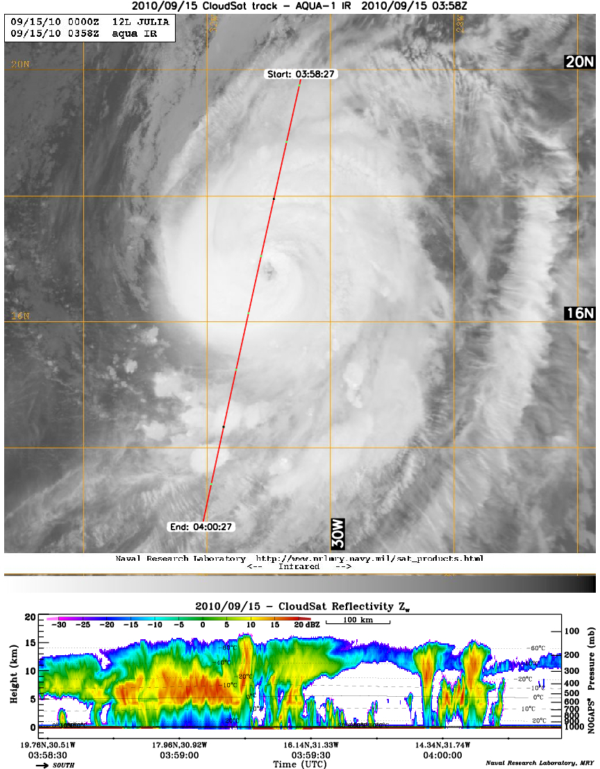
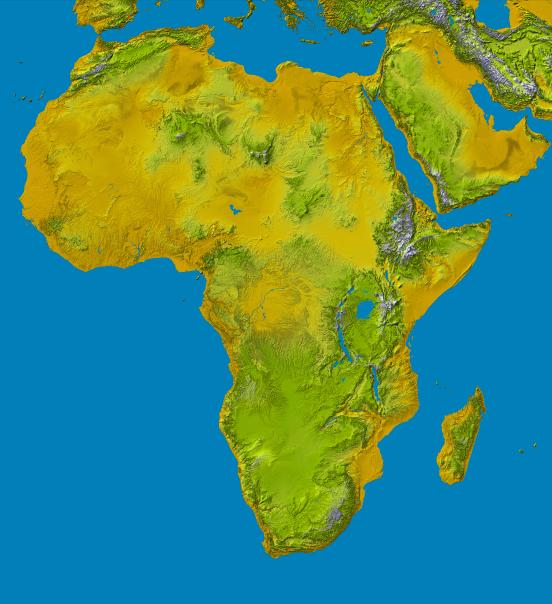
Author information
Authors and Affiliations
Corresponding author
Editor information
Editors and Affiliations
Rights and permissions
Copyright information
© 2017 Springer International Publishing Switzerland
About this entry
Cite this entry
Shimoda, H. (2017). Remote Sensing Data Applications. In: Pelton, J., Madry, S., Camacho-Lara, S. (eds) Handbook of Satellite Applications. Springer, Cham. https://doi.org/10.1007/978-3-319-23386-4_47
Download citation
DOI: https://doi.org/10.1007/978-3-319-23386-4_47
Published:
Publisher Name: Springer, Cham
Print ISBN: 978-3-319-23385-7
Online ISBN: 978-3-319-23386-4
eBook Packages: EngineeringReference Module Computer Science and Engineering