Water Quality Improvement Using Water-Lifting Aeration Technology

Abstract

This chapter introduces the technical background and water quality improvement principles of water-lifting aeration, and describes the methods of designing and optimizing the structure of a water-lifting aerator. The mixing and oxygenation performance of a water-lifting aerator is analyzed using established mathematical models of hydrodynamics and oxygen transfer for the aeration chamber of a water-lifting aerator. Application conditions for controlling the internal water quality pollution and algal blooms by using water-lifting aeration technology are analyzed and discussed. With the help of the computational fluid dynamics (CFD) method, the flow fields outside a water-lifting aerator are numerically simulated, and the effective radius of the algae inhibition zone analyzed and determined. The proper installation height and outflow configuration of a water-lifting aerator are also numerically analyzed and optimized.

1 Introduction of Water-Lifting Aeration Technology

1.1 Background of Water-Lifting Aeration Technology

Eutrophication of lakes and reservoirs has been an important research topic for water scientists and engineers involved with water pollution control and drinking water safety worldwide [1–3]. The main reasons for water eutrophication are point source pollution, such as urban sewage and industrial wastewater, and non-point source pollution, such as agricultural production, soil erosion, and the internal water quality pollution of lakes and reservoirs [4]. Indirect reasons for eutrophication are the hydrological and hydraulic characteristics of lakes and reservoirs. Pollutants such as organic matter, nitrogen, and phosphorus are transported to lakes and reservoirs through rivers [5, 6]. Meanwhile, lakes and reservoirs have the characteristics of large capacity and weak fluidity. Nutrients continue to accumulate in the water and sediment, thereby providing adequate nutrition for algae and other phytoplankton.

Density stratification over the water depth occurs easily in deep-water lakes and reservoirs. Once the water is stratified, the exchange between the upper water and the lower water is limited, and the oxygen concentration in the latter gradually decreases due to the insufficient supply of oxygen. Under anaerobic conditions, a lot of organic and inorganic pollutants can be released from the sediment. The effect of these reactions is a deteriorated aquatic ecological environment [7].

New ideas for in-situ remediation and improvement technologies for lakes and reservoirs having the above-mentioned water quality problems are emerging worldwide [6, 8–12]. They are usually utilized to prevent the occurrence of eutrophication and the release of internal pollutants and to inhibit such problems at the source. In-situ remediation and improvement technologies for lakes and reservoirs have many advantages, such as low investment requirements, working quickly and cleanly with no side effects, and energy-saving operation [13–15].

Mixing and oxygenation using compressed air is one such clean and energy-saving in-situ water quality improvement technology [5, 6, 13, 14, 16–20]. The mixing and oxygenation technology does not add any physical, chemical, or biological issues. Thus, it cannot introduce side effects and does not destroy the aquatic chemical balance or biological environment. There are three main types of in-situ mixing and oxygenation technologies for water quality control, namely, deep aeration–oxygenation, rising plume of air bubbles, and water lifting with pumps or water jets [7].

Deep aeration is also called hypolimnion aeration, by which only the lower water body is oxygenated rather than mixing the upper and lower water bodies. This technology is dedicated to increasing dissolved oxygen in the lower water body and to inhibiting the release of pollutants from sediments [21–24]. However, deep aeration does not spread oxygenated water to the surrounding zone due to small-scale water circulation and it cannot directly control algal growth.

Mixing by bubble plume is achieved by releasing compressed air into the water in the form of small bubbles through diffusers installed at the bottom of lakes and reservoirs [16, 17]. When the air bubbles rise, the lower water is entrained and carried upwards by the bubble plume. Then, it spreads around on the surface area and flows down after local mixing with the surface water, thus forming a kind of vertical circulation. The induced vertical circulation can destroy the thermal stratification [25]. Oxygen is transferred into the water during the bubble flow. Meanwhile, the algae in the surface water can be transported to the middle and lower waters outside of the bubble plume, where the algal growth is inhibited due to the decrease in light intensities and water temperatures [26]. However, the range of the mixing zone is limited, and the requirements for the installation of air tubes are relatively higher, so it is difficult to implement this technology in large deep reservoirs and lakes.

An air-lifting aerator is a straight cylinder with an aeration chamber in its lower part [27]. Compressed air is injected into the aeration chamber, and once the aeration chamber is full, the air will be released instantly, resulting in the formation of a large air piston in the central rising tube and then the plug flows upwards in the straight rising tube. The bottom water is sucked from the lower part of the air-lifting aerator continuously, and is carried upwards in the rising tube. Then, it spreads around on the surface area, leading to the vertical circulation and mixing. The effective mixing area outside the air-lifting aerator is also limited. Currently, the application of this technology lacks any theoretical guidance, which is a considerable problem for its successful application [28]. In addition, air-lifting aeration itself has no function for direct oxygenation.

Recently, the water-lifting aeration technology has been developed for the in-situ water quality improvement and eutrophication control of lakes and reservoirs [5, 6, 13–15, 20, 29]. The water-lifting aerator combines the advantages of the air-lifting aerator, and can mix the upper and lower waters and directly oxygenate the water, expanding its technical capabilities. In recent years, Huang et al. carried out systematic and comprehensive theoretical studies of the structure and performance of water-lifting aerators, as well as an applied study of their control of eutrophication and inhibition of algal growth and pollutant-release from sediments.

1.2 The Water Quality Improvement System of Water-Lifting Aeration

As shown in Fig. 1, the water quality improvement system of water-lifting aeration consists of water-lifting aerators, air compressors, and air conveying pipes.

Fig. 1

Water quality improvement system of water-lifting aeration. (1) Water-lifting aeration, (2) air compressor, (3) air cylinder, (4) prefilter, (5) oil filter, (6) flowmeter, (7) air supply pipeline, (8) cooling water pump

The water-lifting aerators are usually arranged in the entire reservoir or in the vicinity of the reservoir outlet. The distances between water-lifting aerators can be determined by the effective scope of a single water-lifting aerator, which depends on the aerator’s configuration, air flow rate, water depth, and applied purpose of water-lifting aeration. The mechanisms and scope of algae inhibition and destratification are different; the optimization of the water-lifting aeration system can be done by numerical simulation of the hydrodynamics and water quality.

1.3 The Design and Optimization of a Water-Lifting Aerator

Figure 2 shows the diagram of a typical water-lifting aerator. The main part consists of the straight ascending tube installed vertically in the water, along with air supply pipes, an air diffusor, aeration chamber, return chamber, air vessel, water-tight compartment, and anchor pier [20, 30].

Fig. 2

Structural diagram of a water-lifting aerator. (1) Anchor pier, (2) steel chains, (3) air diffusers, (4) aeration chamber, (5) return chamber, (6) air vessel, (7) water-tight compartment, (8) ascending tube, (9) air piston, (10) lock ring, (11) slide tube, (12) air supply pipe, (13) seal plate, (14) overflow plate

The ascending tube is a straight pipe with an inlet near the bottom and an outlet near the surface. The aeration chamber, return chamber, and air vessel are wrapped in the annular space outside the lower section of the ascending tube. The top air vessel is connected to the ascending tube via microholes on the tube’s wall, and the bottom air vessel is separated from the ascending tube by a seal plate. The air-releasing pipe is a circular perforated pipe located below the inlet of the aeration chamber. There is a row of holes with diameters of 2–3 mm downward of the air-releasing pipe. The water-tight compartment is a hollow buoy used to provide buoyancy and to ensure that the water-lifting aerator stands vertically in the water. The anchor pier is a heavy concrete unit resting on the bottom of a reservoir (or lake), used to anchor the water-lifting aerator.

1.3.1 The Structural Design

• 1. Ascending tube

  The ascending tube is a cylindrical straight unit for conveying water flow. The inlet of the ascending tube has a horn-shaped mouth for decreasing the local flow resistance and weakening the disturbance of the sediment by the suction. The vertical distance between the tube’s inlet and the reservoir bottom is nearly 2 m. The outlet of the ascending tube consists of a submerged straight or mushroom tube near the water surface.

  In order to make the water-lifting aerator adapt to any change in water level, the length of the ascending tube can be adjusted automatically. Therefore, the ascending tube can be designed with two segments: the lower segment is fixed to the anchor pier with steel chains and the upper segment is hung below the upper water-tight compartment. The upper segment is connected to the lower segment by a socket. The upper segment is sheathed outside the lower segment, and can float by sliding on the wall of the lower segment. The maximum floating height of the ascending tube is restricted by a ring anchor fixed on the top of the lower segment, as shown in Fig. 2.

• 2. Aeration chamber

  The aeration chamber (Fig. 3a) is divided into three annular zones by the overflow plate and seal plate. The innermost annular zone is surrounded by the vertical seal plate and the central ascending tube’s wall. The two other annular zones are the void air zone and the valid air zone. The air in the valid air zone can flow into the ascending tube and form the air piston. The water level declines as the air is released into the aeration chamber. When the water level drops to the bottom of the seal plate, the air in the top aeration chamber will flow into the ascending tube instantaneously, and the water level in the aeration chamber increases again.

  Fig. 3

  

  Structural graph of the aeration chamber of a water-lifting aerator. (a) Overall configuration of the aeration chamber, (b) detailed configuration of the air outlet slot

  The effective volume of the aeration chamber should be large enough to ensure formatting of the air piston over a certain distance in the rising tube. The diameter of a rising air piston accounts for about 75 % of the ascending tube’s diameter (d). The volume of an air piston must be larger than that of a sphere with a diameter of 0.75d. The effective volume of the aeration chamber also determines the volume of the air piston and the releasing frequency of the air piston, which affects the velocity of the water flow in the rising tube. A detailed analysis of the optimized aeration chamber volume appears in Sect. 3.1.

• 3. Return chamber

  The aeration chamber is a place for air–water contact and oxygen transfer. A circular perforated pipe is installed below the aeration chamber. Released air bubbles are in contact with the water in the aeration chamber, oxygen in the air bubbles is then transferred to the water, and the undissolved air gradually accumulates in the air zones. As the air bubbles rise in the aeration chamber, the water is carried upwards by the rising air bubbles, the anoxic water is then sucked into the aeration chamber through the aerator’s inlet, and the oxygenated water is circulated to the lower zone of the reservoir through the return chamber.

  The bubble plume spreads with a certain width, so the width of the aeration chamber should be less than that of the bubble plume, otherwise, a local circulation can be generated near the aerator’s inlet. In order to control the velocity of water flow downwards in the return chamber and prevent the air bubbles from flowing back to the water through the return chamber, the width and height of the return chamber should be carefully determined. Calculation of the flow rate in the aeration chamber will be described in Sect. 1.3.2.

  In order to weaken the flow fluctuations in the aeration and return chambers, radial separation guide plates are set to separate the annular space. The rising tube, the outer cylinder of the aeration chamber, and the outer cylinder of the return chamber are connected together with the guide plates. Generally, at least four guide plates should be set. Ring baffles are set at the outlet of the return chamber to guide the outflow horizontally and to prevent the formation of a short flow between the outlet of the return chamber and the inlet of the aeration chamber.

• 4. Suspension method

  A water-lifting aerator is suspended in the water with the help of the buoyancy force provided by the water-tight compartment or resin foam. The water-tight compartment is usually made from rigid materials. The lower segment of a water-lifting aerator can slide on the inner wall of the upper segment. If the segments are too long, they should be divided into several subsegments and made separately before installation. The lower subsegments can be connected by a flange and the upper subsegments can be connected using a socket. The upper water-tight compartment is set near the water surface.

1.3.2 Optimization of the Aeration Chamber

• 1. The effects of aeration chamber configuration on the formation of an air piston

  Only when the configuration of the aeration chamber is reasonable can the air piston be formed in the ascending tube by quickly releasing the air in the aeration chamber as a whole. Otherwise, the air in the aeration chamber can only spill in the form of medium-sized air bubbles. The water-lifting performance will be poor if the air piston is not formed. Experimental results show that whether the air piston can be formed depends on the volume of the aeration chamber (V), the width of the air outlet (a), the diameter of the seal plate (D), and the submerged depth of the aeration chamber (H ₀). The greater the V, the smaller the a, D, and H ₀, and the easier it is for the air to overflow one time.

  As shown in Fig. 3b, when the water level drops to the bottom edge of the seal plate, the air pressure inside the seal plate and the water pressure outside the seal plate are equal (P), and then the first air bubble with a volume of ΔV is released. If the original position is filled by the air in the aeration chamber, a continuous bubble flow will then be formed and all the air in the aeration chamber will finally be released. If the original position is filled by the water in the air outflow slot, the residual air in the aeration chamber will then be retained in the chamber and cannot be released after the first bubble.

  Whether the vacated space is filled by the air or the water depends on their respective volumes. If the volume of air in the aeration chamber is greater than that of water in the air outflow slot, the vacated space will be filled by the air in the aeration chamber. The air pressure in the aeration chamber and the water pressure at the bottom edge of the seal plate are equal (P), and the air pressure in the aeration chamber suddenly drops by ΔP ₁, defined as follows:

  $$ \Delta {P}_1=\frac{\Delta V}{V}P. $$

  (1)

  As the first bubble rises, the water pressure near the bubble is less than P. The water pressure drop is marked as ΔP ₂. The greater the ΔV, the greater the ΔP ₂ due to more difficult filling. The greater the water volume in the air outflow slot, the smaller the pressure drop due to easier filling. Therefore, the volume of the air bubble and the width of the air outflow slot can be approximately expressed as follows:

  $$ \Delta {P}_2\propto \frac{\Delta V}{aD}. $$

  (2)

  After the release of the first air bubble, the air pressure in the aeration chamber drops to P – ΔP ₁, and the water pressure near the bubble wake drops to P – ΔP ₂. If the ΔP ₁ is greater than the ΔP ₂, the air pressure in the aeration chamber will be less than the water pressure in the air outlet slot, and the vacated space of the first bubble wake will be filled by the water in the air outflow slot. So, the condition for releasing all the air in the aeration chamber is:

  $$ \Delta {P}_1<\Delta {P}_2. $$

  (3)

• 2. Model of the minimum air chamber volume

  For a specific water depth (H ₀) and diameter of the ascending tube, the width of the air outlet (a) should be chosen to be as small as possible to make the air in the aeration chamber pass through the air outlet within 1–2 s and with an average flow velocity of less than 3–5 m/s. The challenging task of designing the aeration chamber is how to determine the proper volume of the aeration chamber under the conditions of known a, D, and H ₀. Combining Eqs. (1)–(3) yields the following relationship:

  $$ V> kaDP. $$

  The minimum volume of the aeration chamber can be calculated as follows:

  $$ V=k{\left(a+{a}_0\right)}^a{\left(D+{D}_0\right)}^{\beta }{\left(10.3+{H}_0\right)}^{\gamma }+b, $$

  (4)

  where k, a ₀, D ₀, b, α, β, and γ in Eq. (4) are undetermined constants.

  By changing the values of a, D, and H ₀, corresponding values of V can be obtained and the relationship between V and the combined values of a, D, and H ₀ can be developed. The undetermined constants in Eq. (4) can be calibrated against the experimental data using the Marquardt method. After performing programmed computation, the values of the undetermined constants k, c ₀ , D ₀ , b, α, β, and γ are 0.0002, 0.0168, 0.209, 0.001079, 1, 1, and 2.59, respectively.

  The minimum required value of the volume of the aeration chamber (V) can be calculated by substituting values of a, D, and H ₀ in Eq. (4). Figure 4 shows the minimum values of V under different values of a. As shown in Fig. 5, the prediction errors of V are within ±10 %, indicating that the predicted results agree well with the actual results. Thus, the empirical formula expressed with Eq. (4) is feasible and can be used to determine the optimized volume of the aeration chamber.

  Fig. 4

  

  Relationship between V and a

  Fig. 5

  

  Comparison of calculated and measured volumes of the aeration chamber

2 Principles of Water Quality Improvement Using a Water-Lifting Aerator

2.1 Operating Procedures

The operating procedures of a water-lifting aerator are as follows.

Compressed air is continuously released into the aeration chamber through the air diffusers. Some oxygen in the air is transferred to the water as the air rises in the form of microbubbles in the aeration chamber. At the same time, water is carried upwards by air bubbles in the aeration chamber, and the oxygenated water then returns to the reservoir bottom through the return chamber. Undissolved air accumulates in the top zone of the aeration chamber, so the water is forced to flow out from the air zone by the accumulated air, causing the water level to gradually go down in the aeration chamber. When the water level drops to the bottom edge of the seal plate, the air in the aeration chamber will instantaneously pass through the bottom edge of the seal plate and flow into the ascending tube through the air outlet. Then, the aeration chamber will be refilled with water.

Air released from the aeration chamber will combine and form a large air piston in the ascending tube, the air piston will occupy the entire cross-section of the ascending tube and rises quickly, forming a plug flow upwards. The water flow will firstly be accelerated until the air piston goes out of the ascending tube; subsequently, the water flow will be decelerated due to the flow resistance until the formation of the next air piston. The water in the bottom of the reservoir will be sucked by the rising air in the ascending tube and then transported to the surface zone of the reservoir; the water lifted from the reservoir bottom will mix with the water near the reservoir surface and then spread sideways, thus allowing mixing between the upper and lower water layers.

2.2 Principles of Water Quality Improvement

A water-lifting aeration system has direct functions of oxygenating and mixing.

As described in Sect. 2.1, compressed air is released into the water in the aeration chamber, some oxygen in the air bubbles will be transferred to the water in the aeration chamber, and the oxygenated water will return to the reservoir bottom through the return chamber and form a local water circulation in the anoxic bottom zone. The dissolved oxygen concentration is low in the bottom zone and the pressure of the compressed air is high, so high oxygen transfer efficiency can be expected.

Driven by the air piston, the water flow upwards is developed in the ascending tube of a water-lifting aerator, the lower water will be transported to the surface area, and this causes the water flow downwards outside the water-lifting aerator and, hence, water flow upwards inside the aerator and water flow downwards outside the aerator form the circulating water flow in the reservoir. For stratified lakes and reservoirs, when the lower water is transported to the upper zone, the mixture of the lower water and upper water is still heavier than the background upper water, so the upper water will be pushed down gradually. On the other hand, outflow from the aerator will also flow horizontally due to its kinetic energy; this will enlarge the mixing zone and promote the vertical water circulation in a reservoir. Moreover, a strong sucking flow near the inlet of the aeration chamber will then be developed by the pulse flow of high velocity within a short time, and this also affects the water far from the aerator.

Using the water-lifting aeration technology, the oxygen concentration of the lower water can be increased by oxygenating the lower water directly or transporting the upper water of high oxygen concentration by vertical circulation. Once the anoxic condition of the lower water is improved due to increased oxygen concentration, the dissolving and releasing of pollutants from sediment under anaerobic reducing conditions will thus be inhibited. Oxidative decomposition of organic matter in sediment will be promoted.

Most algae mainly grow in the well-lit surface water, and they will sink very slowly after maturation. However, Microcystis aeruginosa, one of the dominant algae in most drinking water reservoirs, can float upwards in the water due to its special buoyancy adjustment mechanism, which gives it more opportunities for growth and reproduction in the surface water. Water circulation generated by water-lifting aeration can be used to control the algal growth by three mechanisms. Firstly, the algae in the surface water can be transported to the lower water by the circulating water flow. They cannot photosynthesize in the dark environment and will gradually die. If the renew rate of the surface water due to the generated circulation is greater than the rate of algal growth, the algae cannot reproduce. Secondly, low temperatures are not conducive to algal growth, so it will be inhibited by the temperature change caused by the water circulation generated by the water-lifting aeration. When the lower water is transported to the surface zone, the temperature of the surface water will fall, so the growth of algae remaining in the surface water will be inhibited. Thirdly, the light penetration will be weakened in the lower water, and this will inhibit the growth of algae.

Air diffusers, the aeration chamber, return chamber, and air vessel are highly integrated in a water-lifting aerator. The water-lifting aerator has functions of oxygenating the lower water and mixing the upper and lower water layers, which can then be used to effectively control the release of pollutants from sediment and the excessive growth of algae in the surface water.

3 Mixing and Oxygenation Performance of a Water-Lifting Aerator

3.1 Water Flow Velocity Model

The water flow rate of a water-lifting aerator directly affects the mixing performance, which is dependent on several factors, such as the air flow rate, the diameter and length of the ascending tube, and the volume of the aeration chamber. This section provides an analysis of the forces acting on the water flow, establishes a mathematical model to calculate the water flow velocity, and provides a validation of the established model.

With the air piston formed intermittently, the water flow velocity in the ascending tube changes periodically. Each cycle of the water flow can be divided into two stages. The first stage is defined as the acceleration stage, in which an air piston is formed and drives water upwards with acceleration until it rushes out of the ascending tube. The second stage is defined as the deceleration stage, in which water in the ascending tube rises with deceleration until the next air slug forms.

3.1.1 Model Development

• 1. Model of water flow velocity in the acceleration stage

  The flow in the acceleration stage is characterized as a gas–liquid two-phase slug flow. When the air piston rises, some water will flow downwards in the form of a water film in the small gap between the air piston and the wall of the ascending tube [31]. The flow of the rising air piston and the water flow are not synchronized; there is a relative sliding movement between the air flow and the water flow. The water between the inlet and outlet of the ascending tube is chosen as a control volume, as shown in Fig. 6.

  Fig. 6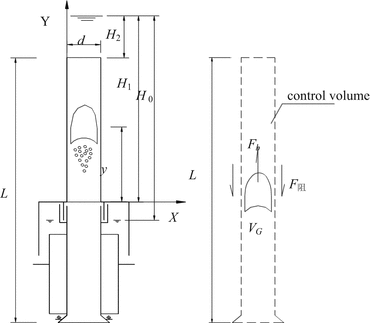

  

  Forces acting on the fluid in the ascending tube of a water-lifting aerator

  In this stage, the buoyancy force and friction resistance act together on the control volume [30]. Using Newton’s second law, the following momentum equation can be obtained:

  $$ F={F}_{\mathrm{b}}-{F}_{\mathrm{f}}=ma=m\frac{d\upsilon }{dt}=m\frac{d\upsilon }{dy}\frac{dy}{dt}=m\upsilon \frac{d\upsilon }{dy}, $$

  (5)

  where F _b is the buoyancy force acting on the control volume from the air piston, N; F _f is the friction resistance acting on the control volume from the wall, N; a is the acceleration of the control volume, m/s²; υ is the rising velocity of the control volume, m/s; y is the height between the air piston and the top of the aeration chamber, m, y ∈ [0, H ₁ – H ₂]; H ₁ is the height between the top of the aeration chamber and the water surface, m; H ₂ is the submerged water depth at the top of the aeration chamber, m; t is the time, s; m is the mass of the control volume, kg.

  The buoyancy force can be expressed as follows:

  $$ {F}_{\mathrm{b}}={V}_{\mathrm{G}}{\rho}_{\mathrm{L}}g, $$

  (6)

  where ρ _L is the water density, kg/m³; g is the gravity acceleration, m/s²; V _G is the volume of the air piston at a specified height, m³.

  The initial volume of the air piston is the effective volume of the air chamber (V ₀), and it will increase due to the reduction of the water pressure as the air piston rises. The rising of the air piston is very rapid; therefore, the expansion of the air piston can be approximately treated as an adiabatic process and expressed as follows:

  $$ {P}_0{V}_0^{1.402}={P}_1{V}_{\mathrm{G}}^{1.402}, $$

  where P ₀ is the absolute air pressure in the aeration chamber, Pa; V ₀ is the effective air volume of the aeration chamber, m³; P ₁ is the absolute pressure of the air piston at a specified height (y), Pa.

  Rearranging the above equation gives:

  $$ {V}_{\mathrm{G}}={V}_0{\left({P}_0/{P}_1\right)}^{1/1.402}={V}_0\frac{{\left(10.33+{H}_0\right)}^{0.713}}{{\left(10.33+{H}_1-y\right)}^{0.713}}, $$

  where H ₀ is the height between the bottom of the aeration chamber and the water surface, m.

  Substituting V _G into Eq. (6) yields the buoyancy force acting on the control volume:

  $$ {F}_{\mathrm{b}}=\frac{{\left(10.33+{H}_0\right)}^{0.713}}{{\left(10.33+{H}_1-y\right)}^{0.713}}{V}_0{\rho}_{\mathrm{L}}g. $$

  (7)

  The friction resistance from the tube’s wall is equal to the water weight equivalent to the water head loss in the ascending tube:

  $$ {F}_{\mathrm{f}}={h}_{\xi }{\rho}_{\mathrm{L}}gA=\left({\zeta}_i+{\zeta}_o+\lambda \frac{L}{d}\right)\frac{\upsilon_{\mathrm{L}}^2}{2g}{\rho}_LgA=\frac{\zeta A{\rho}_{\mathrm{L}}}{2}{\upsilon}_{\mathrm{L}}^2, $$

  (8)

  where h _ξ is the water head loss in the ascending tube, m; A is the cross-sectional area of the ascending tube, m²; ζ _i and ζ _o are the local resistance coefficients of the inlet and outlet of the ascending tube; ζ is the total flow resistance coefficient; L is the length of the ascending tube, m; d is the diameter of the ascending tube, m; υ _L is the water flow velocity, m/s; λ is the friction coefficient of the ascending tube’s wall, relating to the water flow velocity (υ _L)_.

  The mass of the control volume in the ascending tube can be calculated as follows:

  $$ m=\left(V-{V}_{\mathrm{G}}\right){\rho}_{\mathrm{L}}+\frac{10.33+{H}_0}{10.33}{V}_0{\rho}_{\mathrm{G}} $$

  (9)

  where ρ _G is the air density under standard atmospheric pressure, kg/m³; V is the volume of the control volume, m³.

  Substituting Eqs. (7)–(9) into Eq. (5) gives the ordinary differential equation of velocity of the control volume with the height from the top of the aeration chamber to the air piston (y):

  $$ \frac{d\upsilon }{dy}=\frac{B_1{V}_0{\rho}_{\mathrm{L}}g-0.5\zeta A{\rho}_{\mathrm{L}}{\upsilon}_{\mathrm{L}}^2}{\left[\left(V-{B}_1{V}_0\right){\rho}_{\mathrm{L}}+{B}_2{V}_0{\rho}_{\mathrm{G}}\right]\upsilon }, $$

  (10)

  where B ₁ = (10.33 + H ₀)^0.713/(10.33 + H ₁-y)^0.713, B ₂ = 1 + 0.097H ₀.

  The velocity of the air piston (υ _G) is greater than that of the control volume (υ). According to the principle of momentum, the following relationship can be obtained:

  $$ {V}_0{\rho}_{\mathrm{G}}^{\prime }{\upsilon}_{\mathrm{G}}+\left(V-{V}_{\mathrm{G}}\right){\rho}_{\mathrm{L}}{\upsilon}_{\mathrm{L}}=\left({V}_0{\rho}_{\mathrm{G}}^{\prime }+\left(V-{V}_{\mathrm{G}}\right){\rho}_{\mathrm{L}}\right)\upsilon, $$

  (11)

  where ρ ^′_G is the air density at the air pressure in the aeration chamber, kg/m³.

  The velocity of the air piston can be expressed as follows:

  $$ {\upsilon}_{\mathrm{G}}=1.2\upsilon +{\upsilon}_{\infty }, $$

  (12)

  where υ _∞ is the velocity of the air piston in still water:

  $$ {\upsilon}_{\infty }=0.345\sqrt{gd} $$

  Substituting Eqs. (11) and (12) into Eq. (10), the values of υ, υ _G, and υ _L at different values of y and t can be determined by using a numerical differential method.

• 2. Model of the water flow velocity in the deceleration stage

  In the deceleration stage, only friction resistance from the tube’s wall acts on the control volume, the mass of the control volume is constant, and the water flow velocity is equal to the velocity of the control volume. Substituting Eqs. (8) and (9) into Eq. (5) gives the equations of motion of the control volume in the deceleration stage:

  $$ \frac{d{\upsilon}_{\mathrm{L}}}{dt}=-\frac{\zeta }{2L}{\upsilon}_{\mathrm{L}}^2. $$

  (13)

  The integral equation is as follows:

  $$ t=-{\displaystyle {\int}_{\upsilon \max}^{\upsilon_{\mathrm{L}}}\frac{2L}{\zeta {\upsilon}_{\mathrm{L}}^2}}d{\upsilon}_{\mathrm{L}}, $$

  (14)

  where υ _max is the maximum water flow velocity at the end of the acceleration stage.

3.1.2 Model Validation

In order to verify Eqs. (10) and (13), the water flow velocities in the ascending tube at different stages were measured with an ultrasonic flowmeter at a sampling rate of 0.25 s. The measured water flow velocities were compared with the velocities calculated under different conditions. Figure 7 shows the water flow velocities in the ascending tube under two air chamber volumes. The calculated water flow velocities fit the measured values very well, which indicates that the developed water flow velocity models are feasible.

Fig. 7

Water flow velocity with time in the ascending tube of a model water-lifting aerator under different chamber volumes (V ₁ = 17 cm³, V ₂ = 1600 cm³)

3.1.3 Relationship Between Water Flow Rate and Process Parameters

Using the developed mathematical models of water flow velocity, the water flow velocity and water flow rate of a water-lifting aerator can be calculated under different structural and operational parameters. Based on the calculated results, the water flow velocity and water flow rate of a water-lifting aerator monotonically increase with the diameter, length, submerged depth of the aeration chamber, and air flow rate of the aerator. Figure 8 shows the relationship between the average water flow velocity and the air flow rate.

Fig. 8

Relationship between the average water flow velocity and air flow rate Q

The optimum chamber volume V _op is related to the air flow rate Q, length of the water-lifting aerator L (water depth), and chamber position H ₁. For a water-lifting aerator with a certain length and diameter, under a fixed air flow rate, the maximum water flow velocity can be obtained at an optimum chamber volume V _op (Fig. 9).

Fig. 9

Relationship between the average water flow velocity and the effective volume of the aeration chamber V ₀

The relationship equations of the average water flow velocity under different conditions are listed in Table 1.

Table 1 The relationship equations of the average water flow velocity of the ascending tube υ _av (or water flow rate Q _w ) and structural parameters or operational variables of a water-lifting aerator

3.2 Model of Oxygen Transfer in the Aeration Chamber

3.2.1 Model Development

According to the double-film theory, a water film is present on the surface of air bubbles and the oxygen is first transferred to the water film, being in the condition of saturated dissolved oxygen with the concentration of C*, whereas the dissolved oxygen concentration in the main water flow is C. The concentration of the dissolved oxygen gradually increases in the main water flow with increasing water flow (as shown in Fig. 10).

Fig. 10

Simplified diagram of the aeration chamber for studying the oxygen mass transfer model

The dissolved oxygen (DO) concentration is a function of the position z. Taking a thin layer of the aeration chamber with a height of Δz as the control volume, the DO balance in the control volume is analyzed. Assuming that the dissolved oxygen in the control volume is only transferred from the air bubbles, the following DO balance can be expressed:

Total dissolved oxygen out of the control volume = total dissolved oxygen into the control volume + transferred dissolved oxygen from the air bubbles in the control volume.

By setting the dissolved oxygen concentration into the control volume as C, then the dissolved oxygen concentration out of the control volume is $C+\partial C/\partial z\cdot \Delta z.$

The dissolved oxygen transferred from the air film per unit time and per unit volume can be calculated as ${K}_{\mathrm{L}}a\left({C}^{\ast }-C\right)$, where K _L and a are the total area of air bubbles per unit control volume and the oxygen mass transfer coefficient on the gas–liquid interface, respectively.

Setting the cross-sectional area of the aeration chamber as A, the DO balance in the control volume can be expressed as follows:

$$ \left(C+\frac{\partial C}{\partial z}\cdot \Delta z\right)A{U}_{\mathrm{L}}=A{U}_{\mathrm{L}}C+{K}_{\mathrm{L}}a\left({C}^{\ast }-C\right)A\cdot \Delta z. $$

Making Δz→0, transforming the above equation leads to:

$$ \frac{\partial C}{\partial z}=\frac{K_{\mathrm{L}}a}{U_{\mathrm{L}}}\left({C}^{\ast }-C\right), $$

(15)

where C is the DO concentration in water, mg/L; C* is the saturated DO concentration in the water film, mg/L; z is the distance from the calculated position to the bottom of the aeration chamber, m; K _L a is the total mass transfer coefficient, s⁻¹; U _L is the water flow velocity in the aeration chamber, m/s.

According to Henry’s law, the saturated DO concentration in the water film is:

$$ {C}^{\ast }={H}_{\mathrm{A}}{Y}_{\mathrm{A}}P={H}_{\mathrm{A}}{Y}_{\mathrm{A}}\left(1+\frac{H_3-z}{10.33}\right), $$

(16)

where H _A is the Henry’s constant, (mg/L)/atm; Y _A is the oxygen mole fraction in bubbles; P is the total pressure of bubbles, atm; H ₃ is the distance from the bottom of the aeration chamber to the water surface, m.

Assuming that the flow in the aeration chamber is a push flow, then substituting Eq. (16) into Eq. (15) gives:

$$ C=\left({C}_{\mathrm{in}}-{A}_1\right) \exp \left(-{k}_1z\right)-{k}_3z+{A}_1, $$

(17)

where A ₁ = k ₂ + k ₃/k ₁, k ₁ = K _L a/U _L, k ₂ = H _A Y _A/(1 + H ₃/10.33), k ₃ = H _A Y _A/10.33; C _in is the dissolved oxygen concentrations of water at the entrance of the aeration chamber.

In Eq. (17), the unknown parameters are the total mass transfer coefficient K _L a and the water flow velocity in the aeration chamber U _L, and their determination methods will be introduced in Sect. 3.2.2.

3.2.2 Determination of Model Parameters

• 1. The total mass transfer coefficient K _L a

  The total mass transfer coefficient K _L a is related to the air flow rate in the aeration chamber, bubble diameter, water flow velocity, temperature, oxygen diffusion coefficient, and other factors. Referring to the models introduced in the related literature [32], these parameters can be calculated as follows:

  $$ \frac{\Phi}{{\left(1-\Phi \right)}^4}=0.2{(Bo)}^{1/8}{(Ga)}^{1/12}Fr, $$

  (18)
  $$ {d}_{\mathrm{b}}=26{(Bo)}^{-0.5}{(Ga)}^{-0.12}{(Fr)}^{-0.12}D, $$

  (19)
  $$ a=0.33{(Bo)}^{0.5}{(Ga)}^{0.1}{\Phi}^{1.13}{D}^{-1}, $$

  (20)
  $$ {K}_{\mathrm{L}}=0.5{(Se)}^{0.5}{\left( Bo*\right)}^{3/8}{\left( Ga*\right)}^{1/4}{D}_{\mathrm{L}}{d}_{\mathrm{b}}^{-1}, $$

  (21)

  where, Bo, Ga, Fr, Se, Bo*, and Ga* are dimensionless numbers, Bo = (gD ² ρ _L/γ), Ga = (gD ³/v _L ²), $Fr={U}_{\mathrm{G}}/\sqrt{gD}$, Se = (v _L/D _L), Bo* = (gd _b ² ρ _L/γ), and Ga* = (gd _b ³/v _L ²); Ф is the ratio of air bubbles in the mixture of air and water; d _b is the average diameter of air bubbles, m; a is the gas–liquid two-phase contact area per unit volume of water, m²/m³; K _L is the oxygen mass transfer coefficient, m/s; D is the equivalent diameter of the aeration chamber, equal to the square root of the cross-sectional area of the aeration chamber divided by π/4, m; D _L is the molecular diffusion coefficient of oxygen in water, m²/s; v _L is the kinematic viscosity of water, m²/s; γ is the surface tension of water, kg/s²; U _G is the local superficial air flow velocity, equal to the air flow rate divided by the cross-sectional area of the aeration chamber under local conditions, m/s.

  Once the superficial compressed air flow velocity U _G (or flow) in the aeration chamber is known, the cross-sectional area and the total mass transfer coefficient K _L a can be calculated with Eqs. (18)–(21).

• 2. Water flow velocity in the aeration chamber

  The water flow rate in the aeration chamber is directly related to the air flow rate, the height of the aeration chamber, the cross-sectional area of the aeration chamber, and the inlet and outlet forms of the aeration chamber. Referring to the introduced empirical formula in the related literature [32], the water flow rate can be calculated as follows:

  $$ {Q}_{\mathrm{L}}=5.14{h}^{0.698}{Q_{\mathrm{G}}}^{0.459}{5.75}^{D/2}, $$

  (22)

  where Q _L is the water flow rate in the aeration chamber, L/s; h is the height of the aeration chamber, m; Q _G is the air flow rate (converted to that under pressure in the aeration chamber), L/s.

  Laboratory tests were carried out to check the feasibility of Eq. (22). From Table 2, the calculated and measured values of water flow rates in the aeration chamber were basically in agreement, but the calculated water flow rates were larger than those measured in the cases of large air flow rate, which is mainly caused by poor outflow from the return chamber.

  Table 2 Water flow rates in the aeration chamber

  So far, all unknown parameters in Eq. (17) and the increment of the DO concentration between the inlet and outlet of the aeration chamber can be calculated. In order to accurately calculate K _L a and Y _A, the aeration chamber can be divided by several segments in the flow direction, and the segment’s length can be set as 1 m. The values of K _L a and Y _A for each segment can be calculated separately and the oxygen concentration of the front segment’s outlet (C _out) is regarded as that of the following segment (C _in).

3.2.3 Model Validation

• 1. Experimental measurement

  Tap water was first added to a water tank, and aqueous solution of Na₂SO₃ was gradually added. Then, the water in the tank was stirred and the dissolved oxygen concentration was measured until the DO concentration decreased to zero. A water-lifting aerator was put in the water tank and a DO probe was placed at half depth. When operating the water-lifting aerator, the DO concentration in the water tank was measured every 5 min. The total amount of water in the tank was 710 L, the water temperature was 11 °C, and the air flow rates were 800 and 1000 L/h.

• 2. Model calculations

  The inlet DO concentration C _in changed continuously in the aeration chamber, and the increment of dissolved oxygen in the aeration chamber varied with time. After calculation, the water in the water tank could be completely circulated once after 12 periods of releasing the air piston. In order to calculate the oxygen concentration easily, the water tank was simplified to a non-ideal reactor equivalent to 12 completely mixed reactors in series (Fig. 11). A zero-order reaction occurred in 1–12 reactors. According to the principle of mass balance, for the nth reactor, the increment of DO concentration during the time period of Δt is equal to the net amount of DO entering the reactor during Δt, which can be determined by subtracting the amount of outflow from that of inflow in this period. The relationship is as follows:

  $$ {V}_n\left[{C_n}_{\left(t+\Delta t\right)}-{C_n}_{(t)}\right]={C_{n-1}}_{(t)}Q\Delta t-{C_n}_{(t)}Q\Delta t. $$

  Fig. 11

  

  Flume model of non-ideal reactors

  The relationship of dissolved oxygen concentration between any two adjacent reactors in the system of 1–12 reactors can be expressed as follows.

  $$ {C_n}_{\left(t+\Delta t\right)}=\frac{{C_{n-1}}_{(t)}Q\Delta t+{C_n}_{(t)}\left({V}_n-Q\Delta t\right)}{V_n}, $$

  (23)

  where Q is the average flow rate in the water-lifting aerator, C _n is the dissolved oxygen concentration of any reactor in C ₂–C ₁₂; V _n is the volume of the nth aerator.

  C ₁₂ and C ₁₄ are the dissolved oxygen concentrations of the inflow and outflow of the aeration chamber, and their relationship can be expressed with Eq. (17), hence:

  $$ {C}_{14}=\left({C}_{12}-{A}_1\right) \exp \left(-{k}_1z\right)-{k}_3z+{A}_1. $$

  C ₁₃ is obtained by the weighted average of C ₁₂ and C ₁₄:

  $$ {C}_{13}=\frac{Q_{\mathrm{L}}{C}_{14}+\left(Q-{Q}_{\mathrm{L}}\right){C}_{12}}{Q}, $$

  (24)

  where Q _L is the water flow rate in the aeration chamber of a water-lifting aerator, and is calculated by Eq. (22).

  C ₁ is obtained by C₁₃ using Eq. (23).

  At t = 0, C ₁ (0) = C ₂ (0) = … = C ₁₃ (0) = C ₁₄ (0) = 0. Taking the time interval Δt as 1 s, the dissolved oxygen concentration for each reactor can be calculated at different times. A DO analyzer probe is located at the position of #6 reactor. Therefore, the calculated dissolved oxygen concentration of C ₆ is regarded as the measured one in the experiments.

  As can be seen from Fig. 12, the measured values are in good agreement with the calculated values. The measured values are slightly lower only at high dissolved oxygen concentrations. The reason for this is probably excessive dosing of Na₂SO₃. Dissolved oxygen in the water is consumed at high dissolved oxygen concentrations.

  Fig. 12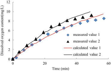

  

  Comparison of calculated and measured dissolved oxygen concentrations under different air flow rates (Q ₁ = 0.8 m³/h, Q ₂ =  1 m³/h)

3.3 Hydrodynamic Model for the Aeration Chamber

In Sect. 3.2, the water flow rate in the aeration chamber was calculated using the proposed empirical model [32]. However, the application of this empirical model is conditional. This section describes a one-dimensional two-phase flow model for the aeration chamber of a water-lifting aerator [33–35]. The model includes the flow rate balance equation, mass conservation equation, momentum balance equation, and energy or pressure balance equation.

3.3.1 Model Development

The aeration chamber can be divided into four parts: the ascending zone, descending zone, the gas–liquid separation zone, and the outflow zone (Fig. 13). The flow in the ascending zone of a chamber is gas–liquid two-phase flow, in which the density of the mixture is less than that of water, and the flow in the descending zone is a single water flow. Driven by the pressure difference caused by the difference inflow density between the ascending zone and the descending zone, the water flows from the ascending zone to the descending zone.

Fig. 13

Diagram of the aeration chamber for studying the hydrodynamic model

A hydraulic model of one-dimensional gas–liquid two-phase flow was established according to the equilibrium between the driving force and drag force acting on the gas–liquid two-phase fluid. The driving force is induced by the gas holdup or density difference between the ascending zone and the descending zone, and the drag force is induced by the wall friction and local flow resistance.

• 1. Balance equation for the ascending zone

  Mass conservation equation:

  $$ {Q}_{lr}={A}_r{V}_{lr}{\varepsilon}_{lr}, $$

  (25)
  $$ {Q}_{gr}={A}_r{V}_{gr}{\varepsilon}_{gr}. $$

  (26)

  The relationship between the superficial velocity and actual velocity is as follows:

  $$ {U}_{gr}={V}_{gr}{\varepsilon}_{gr}, $$

  (27)
  $$ {U}_{lr}={V}_{lr}{\varepsilon}_{lr}. $$

  (28)

  The air flow rate at the air diffusers can be calculated by Eq. (29):

  $$ {Q}_{gr}=\frac{P_{\mathrm{atm}}}{P_{\mathrm{atm}}+{10}^{-5}{\rho}_lg{h}_1^{\hbox{'}}}{Q}_{g\mathrm{atm}}. $$

  (29)

  The pressure drop in the ascending zone includes the gravity pressure reduction and the pressure loss due to the wall friction, and the momentum equation can be expressed as:

  $$ {\left(\frac{dP}{dz}\right)}_r=-\left({\rho}_l{\varepsilon}_{lr}+{\rho}_g{\varepsilon}_{gr}\right)g-{\left(\frac{dP}{dz}\right)}_{fr}. $$

  (30)

  The pressure drop caused by the wall friction in the ascending zone can be expressed as follows:

  $$ {\left(\frac{dP}{dz}\right)}_{fr}=\frac{W_{lr}{\tau}_{plr}}{A_r}. $$

  (31)

  The relationship between the water holdup and the gas holdup is:

  $$ {\varepsilon}_{lr}+{\varepsilon}_{gr}=1. $$

  (32)

  The other equations are:

  $$ {A}_r=\frac{\uppi \left({D}_r^2-{D}_0^2\right)}{4}, $$

  (33)
  $$ {W}_{lr}=\uppi \left({D}_r+{D}_0\right), $$

  (34)

  where Q is the flow rate, m³/s; A is the cross-sectional area, m²; V is the actual velocity, m/s; ε is the gas holdup; U is the superficial velocity, m/s; P is the pressure, N/m²; h ^'₁ is the water depth where the air difussors are located, m; g is the local gravity acceleration, m/s²; ρ is the density, kg/m³; $\frac{dP}{dz}$ is the pressure gradient, Pa/m; τ _p is the shear stress, N/m²; W is the wet perimeter, m; D is the diameter, m.

  The meanings of the subscripts are: r is the ascending zone; d is the descending zone; l is the liquid; g is the gas; atm is the standard atmospheric pressure; f is the wall friction; 0 is the central cylinder.

  Similar equations for the descending zone correspond to Eqs. (25)–(34).

• 2. Local pressure loss

  The pressure loss at the top of the aeration chamber can be expressed as:

  $$ \Delta {P}_{\mathrm{top}}=\frac{1}{2}{\rho}_l{K}_t{V}_{lr}^2. $$

  (35)

  The pressure drop at the outlet of the descending zone can be expressed as:

  $$ \Delta {P}_{\mathrm{out}}=\frac{1}{2}{\rho}_l{K}_E{V}_{lr}^2, $$

  (36)

  where ΔP _top and ΔP _out are the pressure drops caused by the local turning of flow at the top of the ascending zone and at outlet of the descending zone; K _t and K _E are the pressure loss coefficients at the top of the ascending zone and at outlet of the descending zone.

• 3. Relationship of flow rates

  The flow rate in the ascending zone is equal to that in the descending zone:

  $$ {Q}_{lr}={Q}_{ld}\Rightarrow {A}_r{U}_{lr}={A}_d{U}_{ld}. $$

  (37)

• 4. Friction resistance on the wall

  The frictional resistance on the wall of the ascending zone is:

  $$ {\tau}_{plr}=\frac{1}{2}{f}_{lr}{\rho}_l{V}_{lr}^2, $$

  (38)
  $$ {f}_{lr}=0.079R{e}_r^{-0.25}, $$

  (39)
  $$ R{e}_r=\frac{D_{eqr}{V}_{lr}{\rho}_l}{\mu_l}, $$

  (40)

  where f is the friction coefficient; Re is the Reynolds number; μ is the viscosity, kg/(m·s); D _eq is the equivalent diameter to the same cross-section, m.

  The frictional resistance on the wall of the descending zone can also be calculated.

• 5. The energy balance equation or pressure balance equation

  The energy balance or pressure balance of the two-phase flow must be met:

  $$ \Delta {P}_1+{\int}_r\frac{dP}{dz}={\int}_d\frac{dP}{dz}+\Delta {P}_{\mathrm{top}}+\Delta {P}_{\mathrm{out}}. $$

  (41)

• 6. The pressure difference between the inlet and outlet

  The height difference between the inlet and outlet results in the difference of the static pressure caused by potential energy, which can be expressed as:

  $$ \Delta {P}_1={\rho}_lg\left({H}_r-{H}_d\right), $$

  (42)

  where ΔP ₁ is the pressure difference between the inlet and outlet, N/m²; H is the height, m.

  Combining the above equations gives:

  $$ \begin{array}{l}2g\left[\left({\varepsilon}_{ld}+\frac{\rho_g{\varepsilon}_{gd}}{\rho_l}-1\right){H}_d-\left({\varepsilon}_{lr}+\frac{\rho_g{\varepsilon}_{gr}}{\rho_l}-1\right){H}_r\right]\\ {}\kern3.24em =\left(\frac{f_{ld}{W}_{ld}{H}_d{A}_r^2}{A_d^3{\varepsilon}_{ld}^2}+\frac{f_{lr}{W}_{lr}{H}_r}{A_r{\varepsilon}_{lr}^2}\right){U}_{lr}^2+\left({K}_t+{K}_E\right){V}_{lr}^2.\end{array} $$

  (43)

  Since ${\rho}_g<<{\rho}_l,\kern0.24em {\varepsilon}_{gd}<1,\kern0.24em {\varepsilon}_{gr}<1,\kern0.24em \frac{\rho_g{\varepsilon}_{gd}}{\rho_l}\approx 0,\kern0.24em \frac{\rho_g{\varepsilon}_{gr}}{\rho_l}\approx 0.$

  Simplifying Eq. (43) yields:

  $$ 2g\left({\varepsilon}_{gr}{H}_r-{\varepsilon}_{gd}{H}_d\right), $$
  $$ \begin{array}{l}=0.316{\left(\frac{\rho_l}{\mu_l}\right)}^{-0.25}{U}_{lr}^{1.75}\left[{\left(\frac{D_r^2-{D}_o^2}{D_d^2-{D}_r^2}\right)}^{1.75}\frac{{\left({D}_d-{D}_r\right)}^{-1.25}{H}_d}{{\left(1-{\varepsilon}_{gd}\right)}^{1.75}}+\frac{{\left({D}_r-{D}_o\right)}^{-1.25}{H}_r}{{\left(1-{\varepsilon}_{gr}\right)}^{1.75}}\right]\\ {}+\frac{\left({K}_t+{K}_E\right)}{{\left(1-{\varepsilon}_{gr}\right)}^2}{U}_{lr}^2.\end{array} $$

  (44)

  The water flow velocity and gas holdup in the aeration chamber can be predicted from Eq. (44) with the real-domain method of Matlab, but the pressure loss coefficients of K _E and K _t need to be known before using this equation.

  Based on the field data of hypolimnetic aerators installed in Lake Prince and Lake Western Branch, Burris et al. proposed the relationship of ${K}_t=4.7{U}_{lr}^{-1.4}$ [21], and Brodkey and Hershey suggested K _t  = 0.5 [36] according to the experimental results of oxygen transfer. Fried and Idelchick suggested that K _E  = 2.9 (pressure loss coefficient at the inlet of the ascending zone K _in = 1.4, pressure loss coefficient at the outlet of the descending zone K _in = 1.5) [37].

3.3.2 Determination of Model Parameters

Before using use Eq. (44), the relationship between the gas holdup and superficial air velocity and water flow velocity also needs to be developed. The gas holdup in the ascending zone can be calculated with Eq. (45) [38]:

$$ {\varepsilon}_{gr}=\frac{4{Q}_g}{\uppi \left({D}_r^2-{D}_o^2\right)\left({V}_{lr}+{V}_b\right)}=\frac{U_{gr}}{\left({V}_{lr}+{V}_b\right)}. $$

(45)

Wüest et al. also proposed the following relationship between V _b and r _b :

$$ \begin{array}{l}\mathrm{When}\kern0.5em {r}_b<7\times {10}^{-4}\mathrm{m},\kern0.36em {V}_b=4474{r_b}^{1.357};\\ {}\mathrm{When}\kern0.5em 7\times {10}^{-4}\mathrm{m}\le {r}_b\le 5.1\times {10}^{-3}\mathrm{m},\kern0.36em {V}_b=0.23;\\ {}\mathrm{When}\kern0.5em {r}_b>5.1\times {10}^{-3}\mathrm{m},\kern0.36em {V}_b=4.202{r_b}^{0.547},\end{array} $$

where V _b is the rising velocity of air bubbles, m/s; r _b is the radius of air bubbles, m.

As previously described, many empirical equations are combined in the hydrodynamic model for the aeration chamber, so the water flow velocity and gas holdup in the aeration chamber can be accurately predicted with the developed hydrodynamic model by choosing the proper empirical equations according to different experimental conditions.

3.3.3 Model Validation

• 1. Experimental methods

  In order to verify the developed hydrodynamic model for the aeration chamber, a series of experiments were conducted in a model water-lifting aerator. The water flow velocity was measured indirectly with a pitot tube. Pitot tubes were installed at several cross-sections of the descending tube of a lab-scale aerator. Several piezometric tubes were also installed on the outer walls of the ascending zone and descending zone to determine the gas holdups in the ascending zone and descending zone. The nozzles of piezometric tubes and pitot tubes were connected to differential pressure meters with latex hoses to determine the pressure difference.

• 2. Model validation

  Based on the measured water flow velocities and gas holdups and calculated air flow velocities from the air flow rate in the aeration chamber, the gas–liquid two-phase flow drift flux model for these aeration conditions was calibrated with Eq. (46):

  $$ \frac{U_{gr}}{\varepsilon_g}=0.8027\left({U}_{gr}+{U}_{lr}\right)+0.2711. $$

  (46)

  The values of coefficients C ₀ and U _BT are roughly in accordance with those in other related literature.

  Figure 14 shows that the errors of the predicted and measured water flow velocities were within the range of ±15 %. The prediction errors of gas holdup were also within ±15 %. These results indicate that the developed hydrodynamic model has strong applicability to predict the water-lifting performance in an aeration chamber of a water-lifting aerator.

  Fig. 14

  

  Comparison of the measured and predicted superficial water flow velocities in the ascending zone

4 Internal Pollution Control by Water-Lifting Aeration

The water-lifting aeration technology can be used to inhibit the release of contaminants by increasing the dissolved oxygen concentration, which can be achieved by oxygenating the anoxic water and mixing the upper and lower waters. Thus, the premise of using the water-lifting aeration technology is that the bottom water in a reservoir is anoxic or anaerobic. At present, it is generally recognized that the anaerobic condition is the key to the release of pollutants from sediment [4, 7], but the critical dissolved oxygen concentration for the massive release of pollutants from sediment is uncertain. In order to determine the specific application conditions restraining the release of contaminants from sediment using water-lifting aeration, comparative studies were conducted on the releasing rates of pollutants under different conditions of dissolved oxygen concentration.

4.1 Application Condition of Inhibiting the Release of Ammonia Nitrogen

It is always shown to be anaerobic in the sediment; nitrogenous organic matter can be transformed into ammonia nitrogen by the ammonifying bacteria and releasing it into the overlying water [39]. When the overlying water is aerobic, ammonia nitrogen will be transformed into nitrate nitrogen by nitrification, and nitrate nitrogen will seep back to the surface sediment to be transformed into nitrogen by denitrification in a hypoxia state, thus completing the whole process of nitrification and denitrification [40, 41]. However, when the overlying water is anaerobic, ammonia nitrogen released from the sediment can be transformed into nitrate nitrogen smoothly, which will cause the accumulation of ammonia nitrogen [42–44]. What dissolved oxygen concentration in overlying water can hinder the nitration of ammonia nitrogen and cause the accumulation of ammonia nitrogen? The results as shown in Fig. 6 in Sect. 1.1 of Chap. 6 indicate that the accumulation of ammonia nitrogen is caused when the dissolved oxygen concentration in water is less than 2 mg/L. Therefore, the application condition of inhibiting the release of ammonia nitrogen from sediment with water-lifting aeration is a dissolved oxygen concentration less than 2 mg/L.

4.2 Application Condition of Inhibiting the Release of Phosphorus

The release of phosphorus in sediment is not only affected by dissolved oxygen, but is also controlled by the pH value. Experiments of phosphorus release were conducted under combined conditions of different pH values and dissolved oxygen concentrations. The pH values of the three simulated experiments were 6.5, 8, and 9.1, respectively. The dissolved oxygen concentration fell gradually from 5 to 4 mg/L in 20 days, from 4 to 3 mg/L in 10 days, from 3 to 2 mg/L in 10 days, from 2 to 1 mg/L in 12 days, and from 1 to <1 mg/L in 38 days.

In the release experiments, the sediment and water samples were obtained from the main channel of Heihe Reservoir. The algae and other plankton were filtered through a 0.45-μm membrane, eliminating their effects on the experimental results. The reactors, comprising three organic glass columns with diameter and height of 300 mm, were placed in a closed and opaque water tank under a constant temperature of 30 °C. O₂ and N₂ were bubbled into the reactors to maintain the required concentration of dissolved oxygen in the overlying water. The pH value in the overlying water was adjusted with 0.1 M NaOH and HCl solutions.

Figure 15 shows the results of phosphorus concentrations in the overlying water under different experimental conditions.

Fig. 15

Effects of dissolved oxygen concentration and pH on the release of phosphorus

When the pH was 6.5, the concentration of dissolved oxygen decreased from 5 to 1 mg/L in 65 days, and the release rate of phosphorus was zero. When the DO concentration was less than 1 mg/L, phosphorus began to release at an average rate of 9.3 mg/(d m²). This is because the iron combined with phosphorus in sediments was reduced and dissolved (Fe³⁺ → Fe²⁺), and that makes phosphate, which is combined with iron (FePO₄), dissolved, and released into the water. However, the release of phosphorus is unstable [45–47].

When the pH was 8, the release rate of phosphorus during each stage was 1.8, 0.41, 1.21, 0.78, and 16.83 mg/(d m²). The release of phosphorus was caused by the replacement of iron and aluminium phosphate (FePO₄, AlPO₄) with hydroxyl radical (OH⁻) in water. When the DO concentration was less than 1 mg/L, the release of phosphorus was quick, which is the combined result of replacement by OH⁻ and reductive dissolution by iron [30].

When the pH was 9.1, the release rate of phosphorus during each stage was 3.38, 4.64, 4.84, 7.26, and 15.83 mg/(d m²). When the DO concentration decreased from 5 to 2 mg/L, the release rates of phosphorus were stabilized at a low level. This was still the result of the replacement of iron and aluminium phosphate (FePO₄, AlPO₄) by hydroxyl radical (OH⁻) in water. When the DO concentration decreased to 1–2 mg/L, the release of phosphorus was accelerated, indicating that the reductive dissolution by iron began to work. When the DO was less than 1 mg/L, the release of phosphorus was further accelerated, due to the stronger reductive dissolution by iron.

In conclusion, the critical dissolved oxygen concentrations for the anaerobic release of phosphorus are less than 1 mg/L when the pH <8 and less than 2 mg/L when the pH was 9.1. Therefore, under neutral or acidic conditions, the premise of restraining the release of phosphorus from sediments using water-lifting aeration is a dissolved oxygen concentration of less than 1 mg/L, and under alkaline conditions, the premise is a dissolved oxygen concentration less than 2 mg/L.

4.3 Application Condition of Inhibiting the Release of Organic Matter

The release of organic matter from sediment is actually the accumulation of incomplete intermediate byproducts from the decomposition of organic matter under anaerobic conditions. While under aerobic conditions, these intermediate byproducts are decomposed into CO₂ and H₂O. Similar releasing experiments were performed. The dissolved oxygen concentrations were 4 mg/L for 6 days, from 4 to 1–2 mg/L for 6 days, and <1 mg/L for 6 days. The TOC concentrations in water were measured under different conditions of dissolved oxygen concentration. Figure 16 shows the results.

Fig. 16

Effects of dissolved oxygen concentration and pH on the release of organic matter TOC

From Fig. 16, in the aerobic phase of DO >4 mg/L, the TOC concentration in each reactor did not increase but decreased to a certain degree, indicating that organic matter was not released from sediment to overlying water. Under aerobic conditions, aerobic decomposition of organic matter occurred in overlying water, reducing the concentration of organic matter.

In the anoxic stage of DO = 1–2 mg/L, a large amount of organic matter was released from sediment. During this stage of 6 days, the TOC concentration in each reactor significantly increased from 4.3 mg/L to 31.6 mg/L. This shows that, under anoxic conditions of DO = 1–2 mg/L, anaerobic bacteria began to multiply. The insoluble organic matter in sediments was degraded to soluble organic acids, and then released to overlying water. After reaching the state of being completely anaerobic (DO<1 mg/L), the TOC concentration did not further increase in overlying water, but instead decreased. This is because the methane-producing bacteria began to multiply, and the organic acids were biodegraded to methane [30].

The application condition for inhibiting the release of organic matter from sediment using water-lifting aeration is dissolved oxygen concentration less than 2 mg/L.

4.4 Application Conditions of Inhibiting the Release of Iron and Manganese

The release of iron and manganese is by reducing Fe³⁺ and Mn⁴⁺ in the precipitated state to Fe²⁺ and Mn²⁺ in the dissolved state under anaerobic conditions. As described in Sect. 3.4.3, iron and manganese will be rapidly released from sediment when the dissolved oxygen concentration is less than 1 mg/L.

In conclusion, the release of the phosphorus, iron, and manganese from sediment can be inhibited when the DO concentration in the lower water is increased to more than 1 mg/L using water-lifting aeration. The release of ammonia nitrogen and organic matter from sediment can be inhibited simultaneously when the DO is increased to more than 2 mg/L.

5 Algae Inhibition by Water-Lifting Aeration

5.1 Application Conditions of Algae Inhibition

5.1.1 Water Depth

With the help of mixing by water-lifting aeration, the algae in the upper water can be transported to the lower water of a reservoir, and will die due to the unfavorable environment for photosynthetic. The light intensity decreases with increasing water depth, so the production capacity of chlorophyll-a in unit concentration (O₂mg/L/(Chl-a μg/L)) decreases with the increase of water depth. Figure 17 shows the variation of the net production capacity of chlorophyll-a against the water depth. The value of the net production capacity above the compensation point is positive. The area enclosed by the curve above the compensation point and the axes is the positive accumulative net production capacity. And the value of the net production capacity below the compensation point is negative. The area enclosed by the curve below the compensation point and the axes is the negative accumulative net production capacity (respiratory capacity). The summation of the two areas is the net production capacity of the water body when the distribution of the content of chlorophyll-a is uniform and the content is of unit value.

Fig. 17

Productivity of units of chlorophyll-a concentration in relation to depth changes

There are two ways to reduce the net production capacity of water. One is to change the situation where the content of chlorophyll-a in the upper layer is greater than that in the lower layer to one where the distribution of chlorophyll-a in each water layer is uniform. The other is to ensure that the required water is deep enough and to extend the depth of the lower “black zone”, since this can strengthen the algal respiration. Extending the curve plotted in Fig. 17, it can be calculated that the depth needed to achieve zero net production capacity in the water is 12 m. This can be decreased slightly, because of the impact of other factors, such as overcast and rainy weather. In conclusion, the applicable depth for using water-lifting aeration devices to restrain algal growth is at least 10 m.

5.1.2 Mixing Conditions

Microcystis aeruginosa is the dominant species of algae in most drinking water source reservoirs and it can float upwards with a typical velocity of 0.000275 m/s in water [14, 48, 49]. The mechanism of inhibiting algal growth by water-lifting aeration is achieved through a circulated flow from top to bottom caused by water-lifting aeration [20]; the algae are transported to the lower water layer and eventually die due to unfavorable growing conditions. To inhibit the algal growth, a minimum downward flow velocity of 0.000275 m/s is required.

5.2 Spatial Distance Between Two Water-Lifting Aerators

The mixing intensity is great enough to meet the requirements of the downward flow velocity within a certain zone outside a water-lifting aerator. Beyond the certain zone outside a water-lifting aerator, the mixing strength is decreased, and then the algal growth cannot be inhibited. Under certain boundary conditions, the flow field outside a water-lifting aerator can be numerically simulated with the computational fluid dynamics (CFD) method. The powerful CFD simulation software of Fluent can be used [50]. Based on the flow field outside a water-lifting aerator and the typical floating velocity of Microcystis aeruginosa, the effective algae inhibition zones can be numerically determined under different hydrological and operational conditions. Hence, the spatial distance between two water-lifting aerators can be determined.

Based on the typical operational conditions of the water-lifting aeration system used to improve the water quality of Jinpen Reservoir (Fig. 18), the flow field and algae concentration profiles outside the water-lifting aerator under different conditions were numerically simulated, and the effects of the water temperature gradient and water depth on the algae inhibition zone were analyzed [29, 51].

Fig. 18

Layout of water-lifting aerators in Jinpen Reservoir

5.2.1 Simulation Methods

The water body outside the water-lifting aerator was simplified as a two-dimensional axisymmetrical simulation model of the flow domain, and the right half of the simulation model was taken into consideration. The water-lifting aerator was simplified as a cylinder with a radius of 0.375 m, and its central line was set as the axis of the simulation domain. The water-lifting aerator was considered as a block body in which no flow entered or exited. The inlet of the water-lifting aerator was 6 m away from the reservoir bottom and the outlet was 0.5 m below the water surface. The inlet and outlet were considered to be the outlet and inlet of the simulated flow domain, respectively.

Boundary conditions: Velocity-inlet was used to describe the water-inlet of the simulated region. Under typical operational conditions, the velocity increased from 0 to 2.5 m/s linearly within 15 s, then decreased linearly to 0 m/s at 30 s, and then remained at 0 m/s until 270 s in a single cycle [20]. This periodic distribution of velocity was defined by a user-defined function (UDF) of Fluent [52]. The temperature of water-inlet of the simulated region defined by a UDF was the average value of the temperature of water-outlet of the simulation region at the previous simulation time. Pressure-outlet was used to describe the water-outlet of the simulation region and the pressure was decided from the water depth.

Initial conditions: The average water depths before the dam of Jinpen Reservoir are 50–110 m. The observed water temperature in Jinpen Reservoir decreased in linearly from the surface to a depth of 30 m. The seasonal temperature gradients were 0, 0.17, 0.47, and 0.73 °C/m, respectively. The relationship between water temperature and thermal structure, density, and viscosity were defined by a UDF before simulation. The water depths were 50, 80, and 110 m.

Solving methods: The renormalization-group (RNG) κ–ε model was used to model turbulence. The algae concentration was calculated by a multicomponent model. Heat transfer of the surface and subsurface water was considered [53], and the heat transfer conditions were given by the UDF. The first-order upwind scheme was used to discretize the equations, and PISO (pressure implicit splitting of operator) and pressure-based implicit solver were applied to solve the unsteady equations.

Analysis methods of the algae inhibition zone: The zone where the downward vertical velocity is greater than 0.000275 m/s is defined as the core zone of algae inhibition. The area of the zone was calculated using Photoshop software. The percentage of the area of the zone was defined as the ratio of the core zone of algae inhibition to the whole simulation flow domain. The larger the radius of the algae inhibition zone, the better the algae inhibition. The bigger the percentage of the core algae inhibition zone, the better the algae inhibition.

Radius of simulation domain: The preliminary simulated results showed that the core zone of algae inhibition was roughly within 150 m using a water body with a radius of 1600 m. To ensure the reliability and efficiency of the numerical computation, the radius of the subsequent simulation domain was selected as 300 m.

The weakest algae inhibition moment: The preliminary simulated results also showed that the weakest area ratio of the core algal inhibition zone to the whole domain within one period was that at the starting point (endpoint). The following analysis was performed using the starting point data.

5.2.2 Verification of the Simulated Results of Algae Inhibition

The #4 aerator in Jinpen Reservoir was minimally affected by outflow and was taken as the object of verifying the simulated results. A test section was established between #4 and #6 aerators, where the terrain was relatively flat and roughly similar to that of the computational grid. Vertical variations of eight conventional water quality indexes, such as chlorophyll-a and water temperature etc., were measured daily using a Hydrolab DS5X multiprobe sonde (Hach, USA), and algae concentrations of water samples at 0.5 m from the surface, 30 m underwater, and 5 m from the bottom were analyzed in the laboratory twice a week during operation of the aerators. The monitoring profile was 50 m away from #4 aerator.

The flow field outside the water-lifting aerator was measured by three-dimensional acoustic Doppler profilers (ADP, LAUREL company WH600kHz, USA). An ADP measures the flow velocity with the principle of acoustic Doppler [54, 55]. According to the simulated results, the flow out of the aerator was unsteady, and the flow field 50 m away from the aerator was substantially independent of the periodic flow after running for a period of time. Figure 19a shows the simulated algae inhibition zone. Based on the data of vertical flow velocity derived from the ADP, the actual algae inhibition zone is drawn in Fig. 19a. By comparing Fig. 19a, b, the measured and simulated algae inhibition zones were substantially similar, indicating that the simulated vertical velocities and the measured velocities were in good agreement.

Fig. 19

Comparison of the predicted and measured core algae inhibition zones (H = 80 m): (a) predicted zone, (b) measured zone

5.2.3 Effect of Temperature Gradient on the Algae Inhibition Zone

Figure 20 shows the simulated flow fields outside a water-lifting aerator under different temperature gradients.

Fig. 20

Flow fields outside a water-lifting aerator under different water temperature gradients: (a) 0 °C/m, (b) 0.170 °C/m, (c) 0.730 °C/m

The flow field was characterized as a clockwise flow under non-stratified conditions (Fig. 20a); however, the flow field was characterized as a clockwise flow near the domain inlet and a counter-clockwise flow in the other regions under stratified conditions (Fig. 20b, c). Different flow patterns under non-stratified and stratified conditions were mainly caused by the density differences between the inflow and background water. When the water was not stratified, water from the domain inlet initially moved horizontally with its own kinetic energy; a clockwise flow was finally formed outside the aerator under the influence of the right boundary and outlet flow. When the water was stratified, the low-temperature water from the domain inlet initially moved horizontally, and then moved downwards due to its greater density. However, the water flow changed its direction and moved upwards because of the buoyancy resistance from the stratification [56], and, as a result, a partial clockwise flow developed near the domain inlet. The low-temperature water from the domain inlet formed a large counter-clockwise flow on the right side of the aerator.

The temperature gradient affected the flow outside the aerator. When the temperature gradient gradually increased from 0.17 to 0.73 °C/m, the radius of the clockwise flow near the domain inlet decreased from 40 to 25 m, and the maximum velocity of the clockwise flow decreased from 10.5 to 8.5 cm/s. As the kinetic energy of the inflow water and the volume of the water body were all constant, this phenomenon was caused by the difference in buoyancy resistance due to the stratification. As the temperature gradient increased, more energy was consumed when the clockwise flow near the domain inlet moved downwards.

Figure 21 shows the contour lines of the vertical velocity of flow outside the water-lifting aerator, and the colored region is defined as the core zone of algae inhibition.

Fig. 21

Core algae inhibition zones under different temperature gradients: (a) 0 °C/m, (b) 0.170 °C/m, (c) 0.470 °C/m, (d) 0.73 °C/m

The core zone of algae inhibition depended directly on the flow outside the water-lifting aerator; therefore, the shape of the zone under stratified conditions was different from that under non-stratified conditions (Fig. 21). The percentage of the core zone under non-stratified conditions was about 63.95 %, and it increased slightly from 25.2 to 28.6 % when the temperature gradient increased from 0.17 to 0.73 °C/m. The radius of the core inhibition zone increased with the temperature gradient. The radius of the core inhibition zone increased from 100 to 150 m when the temperature gradient increased from 0.17 to 0.73 °C/m. Firstly, a higher temperature gradient led to stronger buoyancy resistance, which restricted the development of clockwise flow near the domain inlet and promoted the development of strong counter-clockwise flow in the other regions. Secondly, as the water temperature at the bottom was almost 6 °C, the water temperature increased with a higher temperature gradient when the upper and bottom waters became completely mixed, and this led to increased water fluidity due to the decreased water viscosity.

5.2.4 Effects of Water Depth on the Algae Inhibition Zone

Figure 22 shows the simulated flow fields outside the water-lifting aerator under water depths of 50, 80, and 110 m. Under a water temperature gradient of 0.73 °C/m, the flow was characterized as a clockwise flow at the inlet and a counter-clockwise flow in other regions, which was similar to that shown in Fig. 20.

Fig. 22

Flow fields outside the water-lifting aerator under different water depths: (a) 50 m, (b) 80 m, (c) 110 m

Figure 22 illustrates that range and strength of the inlet clockwise flow did not changed obviously with water depth. This was because the inlet clockwise flow was mainly influenced by the water temperature gradient, and temperature gradients within the range of 30 m under different depths were identical, and the buoyancy resistance of inlet water with lower temperature was the same too. The vertical velocity of the flow was increased gradually with the increasing water depth, and this was mainly because the ratio of the width to the depth of the water was decreased when the water depth was increased, and the wall effect on the flow structure across the section was gradually enhanced [57].

Figure 23 shows the contour lines of the vertical velocity of flow outside the water-lifting aerator. Although the water depths were different, the shapes of the core zone of algae inhibition were almost the same when the temperature gradient within 30 m was 0.7 °C/m. This was because the core zone depended directly on flow outside the aerator and the flow mainly depended on the temperature gradient. The water depth mainly affected the size of the core zone.

Fig. 23

Core algae inhibition zones under different water depths: (a) 50 m, (b) 65 m, (c) 80 m, (d) 95 m, (e) 110 m

The percentage of the core zone increased from about 12.5 to 30.6 % when the water depth increased from 50 to 110 m. The radius of the core zone increased with water depth. The radius of the core zone increased from about 60 to 175 m when the water depth increased from 50 to 110 m. Because under the condition that the flow domain was not wide enough to limit the flow, the water depth is an important factor affecting the flow when the depth increased within a certain range. Under the condition of constant velocity of the inlet flow, the distance between the inlet and outlet of the flow domain would drive its movement direction to turn left from the right after the inlet flow entered the flow domain outside the aerator. With increasing water depth, the effect of the water outlet became weaker, and the maximum movement distance of the inlet flow gradually increased, manifesting as an increasing core zone of algae inhibition.

Based on the above simulated results, the proper design interval of two water-lifting aerators can be proposed as 250–300 m.

5.3 Installation Height of a Water-Lifting Aerator

The installation height is defined as the vertical distance between the bottom of a water-lifting aerator and the reservoir bottom. To enhance and improve the oxygenation performance of a water-lifting aerator in the bottom water of a reservoir, the installation height should be low. On the other hand, the installation height also influences the suspension of sediment. A proper installation height for a water-lifting aerator needs to be determined.

5.3.1 Simulation Method

To determine the proper installation height of a water-lifting aerator, the flow fields outside a water-lifting aerator under different installation heights were simulated with the Euler–Euler model using Fluent software. The installation heights were 2, 1, and 0.5 m. The water-lifting aerator system installed in Jinpen Reservoir was taken as a study case, and the typical air flow rate of 25 m³/h was used for each simulation case. According to the previous research results of incipient velocity for sediment transport, the water flow velocities above the sediment under different installation heights were compared with the proposed incipient velocity for sediment transport, and the proper installation height of a water-lifting aerator was determined.

5.3.2 Characteristics of Flow Inside and Outside a Water-Lifting Aerator

Under the conditions of an air flow rate of 25 m³/h, a water depth of 80 m, and an installation height of 2 m, the simulated release period of an air piston is about 165 s. The outflow velocity changed periodically within a cycle of about 165 s; it increased linearly from 0 to 4.8 m/s as the time increased from 0 to 15 s, then decreased linearly from 4.8 to 0 m/s as the time increased from 15 to 45 s, and then remained at 0.5 m/s until 165 s.

Because the numerical simulation aimed to evaluate whether the circulated flow can cause the suspension of sediment or not, only the flow fields near the reservoir bottom were analyzed. The bottom water flow is jointly caused by the water flow in the ascending tube and the bubble flow in the aeration chamber of a water-lifting aerator, so the bottom water flow is characterized as the coexistence of multiple circulations, but the flow velocities are usually low due to the large cross-section at the reservoir bottom.

The centerline of the first grid above the reservoir bottom, 0.0795 m from the reservoir bottom, was chosen for analysis of the velocity. Figure 24 shows the temporal variations of the water flow velocity at the specified vertical position. In Fig. 24, the horizontal axis in the figure represents the distance from the water-lifting aerator’s central axis and the time period is one release period of an air piston. Figure 24 shows that the water flow velocity always maximized at a distance of 2 m and always minimized at a distance of 4.25 m.

Fig. 24

Maximum velocities at different aeration times along the centerline of the first grid above the reservoir bottom

To analyze the possibility of the generated water flow disturbing and suspending the bottom sediment, the maximum water flow velocities at the specified vertical position were plotted against the aeration time in Fig. 25. The maximum flow velocity at the specified vertical position varied synchronously with the average flow velocity in the ascending tube of a water-lifting aerator, but the maximum bottom flow velocity was only about 1 % of that in the ascending tube, and the maximum velocity was only 0.0417 m/s.

Fig. 25

Relationship between the maximum velocity along the centerline of the first grid above the reservoir bottom and aeration time (installation height of 2 m)

5.3.3 Flow Characteristics Under Different Installation Heights

Under installation heights of 2, 1, and 0.5 m, the temporal variations of the water flow velocity at the specified vertical position were similar in pattern, but the peak velocities were different. The maximum velocity increased from about 0.02 to 0.23 m/s in 15 s under an installation height of 1 m, but the maximum velocity increased from about 0.1 to 2.1 m/s in 15 s under an installation height of 0.5 m. From Figs. 25 and 26, the maximum water flow velocities at the centerline of the first grid above the reservoir bottom under installation heights of 2, 1, and 0.5 m were about 0.041, 0.23, and 2.1 m/s, respectively.

Fig. 26

Relationship between the maximum velocity along the centerline of the first grid above the reservoir bottom and aeration time: (a) installation height of 1 m, (b) installation height of 0.5 m

5.3.4 Proper Installation Height

At present, the incipient movement of sediment is usually evaluated by three methods, namely, the incipient friction velocity formula, the incipient shear stress formula, and the incipient velocity formula. As shown in Fig. 27, the incipient velocity is dependent on the diameter of the sediment and minimizes in the diameter range of 0.1–1 mm [58]. Under a typical air flow rate of 25 m³/h, the maximum water flow velocities were 0.042, 0.22, and 2.1 m/s for installation heights of 2, 1, and 0.5 m, respectively. Based on the incipient velocities as shown in Fig. 27, it can be deduced that running water-lifting aerators with installation heights greater than 1 m will not cause the suspension and movement of reservoir sediment, regardless of the sediment diameter, which will not increase the water turbidity and deteriorate the water quality of the reservoir. Considering the actual geometry of the reservoir bottom, the installation technology, and the total comprehensive installation cost, the proper installation height of a water-lifting aerator can be suggested as 2 m.

Fig. 27

Relationship between the incipient velocity and sediment diameter

5.4 Effects of Water-Lifting Aerator Type on Algae Inhibition

Two types of water-lifting aerators have been developed to improve the water quality in reservoirs: submerged [13, 20] and non-submerged [5, 6]. From the perspective of economic costs, the initial investment and operating costs of a submerged aerator are about one-third of that of a non-submerged aerator. Moreover, it is also easier to install and maintain. From the perspective of water quality improvement, the function of hypolimnetic aeration is the same for each type of aerator, but the mixing between the upper and lower water bodies will be different, so the effectiveness of mixing as a means of algae inhibition will also be different for the two types of aerator.

To choose the proper type of water-lifting aerator, the effectiveness of algae were numerically compared using non-submerged and submerged water-lifting aerators under the same operational conditions [15, 35]. A water-lifting aerator with an optimized outlet configuration was used. The water depths were 77.25, 87.25, and 97.25 m. The outlet of the submerged aerator was 70 m above the domain bottom and the outlet of the non-submerged aerator was 1.1 m below the water surface. The other simulation methods are the same as those in previous sections.

5.4.1 Algae Inhibition Under Non-stratified Conditions

Figure 28 shows the contour lines of the vertical velocity of flow outside the water-lifting aerators, with the colored region defined as the core algae inhibition zone. From Fig. 28, when the water depth was increased from 77.25 to 97.25 m, the percentage of the core algae inhibition zone to the whole domain was decreased from 56.01 to 47.34 % for the submerged case, while that for the non-submerged case was decreased from 55.48 to 40.15 %. This indicates that the percentage of the core algae inhibition zone for the submerged case is larger than that for the non-submerged case under each water depth. That is because the water from the outlet of the submerged aerator interacts with the background water in the domain from the depth of 77.25 m, which is wider in space and earlier in time than for the non-submerged case; the clockwise flow initially generated from entrainment develops laterally in a wider area. On the contrary, the water from the outlet of the non-submerged aerator interacts with the background water in a narrower area. As the input energy is fixed, the core algae inhibition zone is pushed closer to the right wall of the domain.

Fig. 28

Core algae inhibition zones outside submerged and non-submerged water-lifting aerators at different water depths: (a) submerged, H = 77.25 m, (b) non-submerged, H = 77.25 m, (c) submerged, H = 87.25 m, (d) non-submerged, H = 87.25 m, (e) submerged, H = 97.25 m, (f) non-submerged, H = 97.25 m

It can also be seen from Fig. 28 that the area of the core algae inhibition zone was obviously decreased with increasing depth. The main reason for this is that the boundary effect becomes more evident as the ratio of the depth to the width increases. The stronger the boundary effect, the bigger the vertical velocity, hence the closer the core algae inhibition zone is to the right wall.

5.4.2 Algae Inhibition Under Stratified Conditions

In the study, Jinpen Reservoir is a typical stratified reservoir [5, 6]. The thermocline lies between depths of 0 and 30 m, the temperature reduced from 28 to 6 °C when the depth increased from the water surface to 30 m, the zone below 30 m was an isothermal layer, with the temperature there remaining at 6 °C, and the temperature gradient was 0.73 °C/m.

• 1. Effects of aerator type on the core algae inhibition zone

  Figure 29 shows the simulated core algae inhibition zone under different water depths, with the colored region defined as the core algae inhibition zone. From Fig. 29, when the water depths were 77.25, 87.25, and 97.25 m in the submerged water-lifting aerator case, the percentages of the core algae inhibition zones to the whole flow domain were 39.71, 41.14, and 42.73 %, respectively. For the non-submerged water-lifting aerator case, the percentages were 33.83, 37.46, and 41.58 %, respectively. This indicates that the percentage of the core algae inhibition zone for the submerged case was larger than that for the non-submerged case at each water depth. This is because the core algae inhibition zone is mainly determined by the velocity field. The effect of aerator type on the core algae inhibition zone was consistent with the effect on the flow outside the water-lifting aerators.

  Fig. 29

  

  Core algae inhibition zones outside submerged and non-submerged water-lifting aerators at different water depths: (a) submerged, H = 77.25 m, (b) non-submerged, H = 77.25 m, (c) submerged, H = 87.25 m, (d) non-submerged, H = 87.25 m, (e) submerged, H = 97.25 m, (f) non-submerged, H = 97.25 m

  Figure 29 also shows that the core algae inhibition zone area increased with increasing depth. The main reason for this is that, when the width cannot sufficiently limit the development of the circulation, the water depth acts as a major factor affecting the flow development. For a non-submerged aerator, when the inlet velocity was certain, the water flow from the inlet of the domain was equivalent to a horizontal jet, the distance between the inlet and the bottom would affect the direction of motion, and with increasing water depth, the maximum distance of movement rightward of the inlet flow increased accordingly, which was manifested as the enlargement of the core algae inhibition zone area. For the submerged type, the upper surface was the main factor limiting the flow development, so the deeper the water, the weaker the effect of the upper surface and the further the flow circulation developed.

• 2. Mixing time of algae

  The algae concentration decreasing to a constant value was taken as a sign of complete mixing of algae. The times required for complete algal mixing in three vertical directions and one lateral direction were analyzed. The distances were 20, 100, and 200 m from the aerator and 3 m below the water surface, respectively. As shown in Fig. 30, the x-axis represents the running time in hours. In Fig. 30a–c, the y-axis represents the simulated average algae concentration in the vertical direction, while in Fig. 30d, it represents the simulated average algae concentration in the horizontal direction. In the submerged aerator case, the times required for complete algal mixing in the three water depth conditions were roughly 10, 12, and 14 days, respectively. In the non-submerged case, the corresponding times were about 18, 19, and 20 days, respectively. In the non-submerged case, a longer time was needed for algae to completely mix compared to that in the submerged case. Complete mixing of algae in the submerged case could be achieved earlier, an effect that was very obvious in the vertical direction.

  Fig. 30

  

  Simulated times required for algae to completely mix for different aerator types: (a) 20 m horizontally from the aerator, (b) 100 m horizontally from the aerator, (c) 200 m horizontally from the aerator, (d) 3 m below the water surface

  Therefore, as shown in Fig. 30a–c, the greater the water depth, the lower the algae concentration after complete mixing. In addition, at the beginning, the nearer to the aerator, the higher the algae concentration. That is because, in early operation, the circulation near the aerator side of the velocity field was small, influenced by the flow circulation. Algae far from the aerator were swept closer, so the algae concentration in the area close to the aerator was larger. For the adaptability of the flow, the water circulation to the right would react to the movement of the circulation near the aerator and spontaneously supplement the area near the aerator, where the algae concentration was lower, so the algae concentration in this flow area far from the aerator was further diluted. With the circulation developing more widely, the mixing of algae was more efficiently characterized by the algae concentration tending to be stable in every direction. As can be seen from Fig. 30d, the algae fraction near the surface was effectively reduced.

  Considering the advantages of more effective algal inhibition, lower initial investment, and easier operational management, the submerged water-lifting aerator was suggested for engineering applications in stratified reservoirs.

References

Kraus TEC, Bergamaschi BA, Hernes PJ et al (2011) How reservoirs alter drinking water quality: organic matter sources, sinks, and transformations. Lake Reservoir Manage 27(3):205–219
Lui YS, Hong HC, Zheng GJS et al (2012) Fractionated algal organic materials as precursors of disinfection by-products and mutagens upon chlorination. J Hazard Mater 209:278–284
Zhang P, Zhai CM, Chen RQ et al (2012) The dynamics of the water bloom-forming Microcystis aeruginosa and its relationship with biotic and abiotic factors in Lake Taihu, China. Ecol Eng 47:274–277
Huang TL, Cong HB, Chai BB (2009) Source water quality pollution and control. China Architecture & Building Press, Beijing
Huang TL, Li X, Rijnaarts H et al (2014) Effects of storm runoff on the thermal regime and water quality of a deep, stratified reservoir in a temperate monsoon zone, in Northwest China. Sci Total Environ 485–486:820–827
Huang TL, Ma Y, Cong HB et al (2014) Application of the technology of water lifting and aeration on improving water quality in a Deep Canyon Reservoir – a case study from northern China. Desalin Water Treat 52(7–9):1636–1646
Sun X, Huang TL (2013) Water pollution control of lakes and reservoirs. Hubei Scientific and Technical Press, Wuhan
Lawson R, Anderson MA (2007) Stratification and mixing in lake Elsinore, California: an assessment of axial flow pumps for improving water quality in a shallow eutrophic lake. Water Res 41(19):4457–4467
Xu Y, Yang J, Ou M et al (2007) Study of Microcystis aeruginosa inhibition by electrochemical method. Biochem Eng J 36(3):215–220
Kotopoulis S, Schommartz A, Postema M (2009) Sonic cracking of blue-green algae. Appl Acoust 70(10):1306–1312
Cao CJ, Zheng BH, Chen ZL (2011) Eutrophication and algal blooms in channel type reservoirs: a novel enclosure experiment by changing light intensity. J Environ Sci 23(10):1660–1670
Lundgren VM, Roelke DL, Grover JP et al (2013) Interplay between ambient surface water mixing and manipulated hydraulic flushing: implications for harmful algal bloom mitigation. Ecol Eng 60:289–298
Cong HB, Huang TL, Chai BB (2009) A new mixing–oxygenating technology for water quality improvement of urban water source and its implication in a reservoir. Renew Energy 34(9):2054–2060
Cong HB, Huang TL, Chai BB (2011) Research on applying a water-lifting aerator to inhibit the growth of algae in a source-water reservoir. Int J Environ Pollut 45(1–3):66–175
Sun X, Li XL, Zhang MD et al (2014) Comparison of water-lifting aerator type for algae inhibition in stratified source water reservoirs. Ecol Eng 73(12):624–634
Heo WM, Kim B (2004) The effect of artificial destratification on phytoplankton in a reservoir. Hydrobiologia 524(1):229–239
Liu L, Liu D, Johnson DM et al (2012) Effects of vertical mixing on phytoplankton blooms in Xiangxi Bay of Three Gorges Reservoir. Water Res 46(7):2121–2130
Simmons J (1998) Algal control and destratification at Hanningfield reservoir. Water Sci Technol 37(2):309–316
Jungo E, Visser PM, Stroom J (2001) Artificial mixing to reduce growth of the blue-green alga Microcystis in Lake Nieuwe Meer, Amsterdam: an evaluation of 7 years of experience. Water Sci Technol Water Supply 1(1):17–23
Cong HB, Huang TL, Chai BB (2011) Water-circulating aerator: optimizing structure and predicting water flow rate and oxygen transfer. J Hydraul Eng 137(6):659–667
Burris VL, Mcginnis DF, Little JC (2002) Predicting oxygen transfer and water velocity in airlift aerators. Water Res 36(18):4605–4615
Gantzer PA, Bryant LD, Little JC (2009) Effect of hypolimnetic oxygenation on oxygen depletion rates in two water-supply reservoirs. Water Res 43(6):1700–1710
Bryant LD, Hsu-Kim H, Gantzer PA et al (2011) Solving the problem at the source: controlling Mn release at the sediment–water interface via hypolimnetic oxygenation. Water Res 45(19):6381–6392
Tofflon M, Ragazzi M, Righetti M et al (2013) Effects of artificial hypolimnetic oxygenation in a shallow lake. Part 1: phenomenological description and management. J Environ Manage 114:520–529
Zboray R, Cachard FD (2005) Simulating large-scale bubble plumes using various closure and two-phase turbulence models. Nucl Eng Des 235(8):867–884
Visser PM, Ketelaars HAM, Mur LR (1995) Reduced growth of the cyanobacterium microcystis in an artificially mixed lake and reservoir. Water Sci Technol 32(4):53–54
Goldyn R, Podsiadlowski S, Dondajewska R et al (2014) The sustainable restoration of lakes—towards the challenges of the Water Framework Directive. Ecohydrol Hydrobiol 14(1):68–74
Seo D, Jang DS, Kwon OH (1995) The evaluation of effects of artificial circulation on Daechung Lake, Korea. In: Proceedings of 6th international conference on the conservation and management of lakes, vol 11. pp 336–339
Sun X, Xu Y, Wang X et al (2014) Effects of water depth on algae control in stratified reservoirs by in-situ water-lifting aeration technology. Acta Sci Circumst 34(5):1166–1172
Cong HB (2007) Studies on source water quality improvement technology of water-lifting and aeration. Dissertation, Xi’an University of Architecture and Technology
Zhang YJ, Wang HY, Zhang ZP (1987) Two-phase fluid dynamics. Beihang University Press, Beijing
Little JC (1995) Hypolimnetic aerators: predicting oxygen transfer and hydrodynamics. Water Res 29(11):2475–2482
Zhang WS (2009) Modeling and Simulating of oxygen transfer and water flow rate in the aeration chamber of Water-lifting Aerator. Dissertation, Xi’an University of Architecture and Technology
Sun X, Duan FF, Huang TL et al (2013) Development and sensitivity analysis of model for aeration chamber in water-circulating aerator. Appl Mech Mater 261–262:663–668
Sun X, Zhang MD, Zhao WL et al (2013) Comparison of water-lifting aerator type for algae inhibition in deep reservoirs. Appl Mech Mater 295–298:1053–1056
Brodkey RS, Hershey HC (1988) Transport phenomena-a unified approach. McGraw-Hill, New York
Fried E, Idelchick IE (1989) Flow resistance: a design guide for engineers. Hemisphere Publishing, New York
Wüest A, Brooks NH, Imboden DM (1992) Bubble plume modeling for lake restoration. Water Resour Res 28:3235–3250
Trimmer M, Nicholls JC, Deflandre B (2003) Anaerobic ammonium oxidation measured in sediment along the Thames estuary, United Kingdom. Appl Environ Microbiol 69(11):6447–6454
Zehr JP, Ward BB (2002) Nitrogen cycling in the ocean: new perspectives on processes and paradigms. Appl Environ Microbiol 68(3):1015–1024
Casey RE, Taylor MD, Klaine SJ (2004) Localization of denitrification activity in macropores of a riparian wetland. Soil Biol Biochem 36:563–569
Boatman CD, Murray JW (1982) Modeling exchangeable NH4+ adsorption in marine sediments: process and controls of adsorption. Limnol Oceanogr 27:99–100
Morin J, Morse JW (1999) Ammonium release from re-suspended sediment in the Laguna Madre estuary. Mar Chem 65:97–100
Beutel MW (2006) Inhibition of ammonia release from anoxic profundal sediments in lakes using hypolimnetic oxygenation. Ecol Eng 28(3):271–279
Bostom B, Andersen JM, Fleischer S, Jansson M (1988) Exchange of phosphorus across the sediment–water interface. Hydrobiologia 170:229–244
Kim LH, Choi E, Stenstrom MK (2003) Sediment characteristics, phosphorus types and phosphorus release rates between river and lake sediments. Chemosphere 50:53–61
Kim LH, Choi E, Gil KI et al (2004) Phosphorus release rates from sediments and pollutant characteristics in Han River, Seoul, Korea. Sci Total Environ 321:115–125
Cao HS, Tao Y, Kong FX et al (2008) Relationship between temperature and cyanobacterial recruitment from sediments in laboratory and field studies. J Freshw Ecol 23:405–412
Catherine Q, Susannac W, Isidoraa ES et al (2013) A review of current knowledge on toxic benthic freshwater cyanobacteria – ecology, toxin production and risk management. Water Res 47(15):5464–5479
Fluent Inc. (2006) FLUENT user’s guide. Fluent Inc.
Sun X, Ye LL, Zhao WL et al (2014) Effect of temperature gradient on algal inhibition by in-situ water-lifting aeration in a stratified reservoir. China Environ Sci 34(2):352–358
Fluent Inc. (2006b) FLUENT user defined function manual. Fluent Inc.
Hodges BR (1999) Heat budget and thermodynamics at a free surface. Centre for Water Research, The University of Western Australia
Sun X, Shiono K, Chandler JH et al (2010) Discharge estimation in small irregular river using LSPIV. Proc Inst Civ Eng Water Manage 163(5):247–254
Gunawan B, Sun X, Sterling M (2012) The application of LS-PIV to a small irregular river for inbank and overbank flows. Flow Meas Instrum 24:1–12
Fischer HB, List JE, Koh CR et al (1979) Mixing in inland and coastal waters. Academic Press, London
Sun X, Shiono K (2009) Flow resistance of one-line emergent vegetation along the floodplain edge of a compound open channel. Adv Water Resour 32(3):430–438
Dou GR (1999) Incipient motion of coarse and fine sediment. Shuili Xuebao/J Hydraul Eng 6:1–9
Author information
Authors and Affiliations
Corresponding author
Editor information
Editors and Affiliations
Rights and permissions
Copyright information
© 2016 Springer International Publishing Switzerland
About this chapter
Cite this chapter
Huang, T., Sun, X., Li, X., Cong, H., Cheng, Y. (2016). Water Quality Improvement Using Water-Lifting Aeration Technology. In: Huang, T. (eds) Water Pollution and Water Quality Control of Selected Chinese Reservoir Basins. The Handbook of Environmental Chemistry, vol 38. Springer, Cham. https://doi.org/10.1007/978-3-319-20391-1_9
Download citation
DOI: https://doi.org/10.1007/978-3-319-20391-1_9
Publisher Name: Springer, Cham
Print ISBN: 978-3-319-20390-4
Online ISBN: 978-3-319-20391-1
eBook Packages: Earth and Environmental ScienceEarth and Environmental Science (R0)