
Abstract
This article studies the relationship between loadings from factor analysis (FA) and principal component analysis (PCA) when the number of variables p is large. Using the average squared canonical correlation between two matrices as a measure of closeness, results indicate that the average squared canonical correlation between the sample loading matrix from FA and that from PCA approaches 1 as p increases, while the ratio of p/N does not need to approach zero. Thus, the two methods still yield similar results with high-dimensional data. The Fisher-z transformed average canonical correlation between the two loading matrices and the logarithm of p is almost perfectly linearly related.
Access provided by Autonomous University of Puebla. Download conference paper PDF
Keywords
- Canonical correlation
- Factor indeterminacy
- Fisher-z transformation
- Guttman condition
- Large p small N
- Ridge factor analysis
15.1 Introduction
Factor analysis (FA) and principal component analysis (PCA) are frequently used multivariate statistical methods for data reduction. In FA (Anderson 2003; Lawley and Maxwell 1971), the p-dimensional mean-centered vector of the observed variables y is linearly related to an m-dimensional vector of latent factors f as \( \boldsymbol{y}=\boldsymbol{\Lambda} \boldsymbol{f}+\boldsymbol{\varepsilon} \), where Λ is the p × m matrix of factor loadings (with p > m), and ε is a p-dimensional vector of errors. Typically for the orthogonal factor model, the three assumptions are imposed: (1) \( \boldsymbol{f}\sim {N}_m\left(\mathbf{0},{\boldsymbol{I}}_m\right) \); (2) \( \boldsymbol{\varepsilon} \sim {N}_p\left(\mathbf{0},\boldsymbol{\Psi} \right) \), where Ψ is a diagonal matrix; (3) \( Cov\left(\boldsymbol{f},\boldsymbol{\varepsilon} \right)=\mathbf{0} \). Then, under these three assumptions, the covariance matrix of y is given by \( \boldsymbol{\Sigma} =\boldsymbol{\Lambda} \boldsymbol{\Lambda}'+\boldsymbol{\Psi} \).
Let \( {\boldsymbol{\Lambda}}^{+} \) be the p × m matrix whose columns are the standardized eigenvectors corresponding to the first m largest eigenvalues of Σ; Ω be the m × m diagonal matrix whose diagonal elements are the first m largest eigenvalues of Σ; and Ω 1/2 be the m × m diagonal matrix whose diagonal elements are the square root of those in Ω. Then principal components (PCs) (c.f., Anderson 2003) with m elements are obtained as \( {\boldsymbol{f}}^{*}={\boldsymbol{\Lambda}}^{+\prime}\boldsymbol{y} \). Clearly, the PCs are uncorrelated with a covariance matrix \( {\boldsymbol{\Lambda}}^{+\prime}\boldsymbol{\Sigma} {\boldsymbol{\Lambda}}^{+} \). When m is properly chosen, there exists \( \boldsymbol{\Sigma} \approx {\boldsymbol{\Lambda}}^{+}\boldsymbol{\Omega} {\boldsymbol{\Lambda}}^{+\prime}={\boldsymbol{\Lambda}}^{*}{\boldsymbol{\Lambda}}^{*\prime} \), where \( {\boldsymbol{\Lambda}}^{*}={\boldsymbol{\Lambda}}^{+}{\boldsymbol{\Omega}}^{1/2} \) is the p × m matrix of PCA loadings.
It has been well known that FA and PCA often yield approximately the same results, especially their loading matrices \( \widehat{\boldsymbol{\Lambda}} \) and \( {\widehat{\boldsymbol{\Lambda}}}^{*} \), respectively. See, e.g., Velicer and Jackson (1990) and the literature cited therein. Conditions under which the two matrices are close to each other are of substantial interest. At the population level, one such condition identified by Guttman (1956) requires that \( p\to \infty \) while \( m/p\to 0 \). For the one-factor model with \( \boldsymbol{\Lambda} = \boldsymbol{\lambda} \) and \( {\boldsymbol{\Lambda}}^{*} = {\boldsymbol{\lambda}}^{*} \), under the conditions that \( \boldsymbol{\lambda}^{\prime}\boldsymbol{\lambda} \to \infty \) and there exists an upper bound for unique variances as \( p\to \infty \), Bentler and Kano (1990) proved that λ converges to λ. Let ψ max be the largest element of the diagonal matrix Ψ of unique variances, d min be the smallest eigenvalue of Λ ′ Λ, and
be the average squared canonical correlation between Λ and Λ *. Schneeweiss and Mathes (1995) showed that \( {\rho}^2\left(\boldsymbol{\Lambda}, {\boldsymbol{\Lambda}}^{*}\right)\to 1 \) if \( {\psi}_{\max }/{d}_{\min}\to 0 \). Schneeweiss (1997) further gave a weaker condition: \( \delta /{d}_{\min}\to 0 \) where \( \delta ={\psi}_{\max }-{\psi}_{\min } \) is the difference between the largest and the smallest diagonal element of Ψ. Here, note that Guttman’s condition is expressed by only p and m, and the role of FA loadings is not mentioned. On the other hand, Schneeweiss-Mathes and Schneeweiss conditions are expressed in terms of the eigenvalue(s) of FA loadings and unique variance(s), and the roles of p and m are not mentioned. Yet, it is known that both are closely related (Hayashi and Bentler 2000; Krijnen 2006).
Recently, with the advancement of computing technology, high-dimensional data with large p arise in many disciplines (see, e.g., Hastie et al. 2009). Consequently, the needs for improving our statistical methodology for analyzing such data are increasing. Large p is also common in the traditional research in social sciences. For example, the Minnesota Multiphasic Personality Inventory-2 (MMPI-2; Butcher et al. 1989) contains 567 items, and the scale has been widely used to assess individual mental health. (Note that MMPI-2 items are binary and we must apply FA for ordered categorical data. In our study, we focus on FA for continuous data.) Also, we often collect data from many questionnaires. As a result, whenever we consider item analysis with multiple questionnaires combined, we have to face the issue of analyzing high-dimensional data. Recently, under high-dimensional setting and when both p and N approach infinity, Bai and Li (2012) studied FA and PCA, and showed that their loading estimates converge to the same asymptotic normal distribution, where an additional assumption of \( \sqrt{p}/N\to\ 0 \) is needed.
Although some authors called data with p > N as high-dimensional (see, e.g., Hastie et al. 2009, Chapter 18; Pourahmadi 2013), we do not require this assumption to accommodate typical social science data. Also, we do not consider covariance matrix that has many zero entries, called sparsity (see, e.g., Buehlmann van de Geer 2011).
15.2 Purpose of Study
We examine the closeness of the estimates of the two loading matrices from FA and PCA under high-dimensional setting. Thus, the main goal of our work is to investigate whether the closeness measured by the average squared sample canonical correlation \( {\rho}^2\left(\widehat{\boldsymbol{\Lambda}},{\widehat{\boldsymbol{\Lambda}}}^{*}\right) \) approaches 1 under the conditions analytically derived by Guttman (1956), Schneeweiss and Mathes (1995), and Schneeweiss (1997); and also under high-dimensional setting with large p when N is relatively small.
Notice that Schneeweiss and Mathes (1995) and Schneeweiss (1997) only considered the population loading matrices without any sampling errors. In contrast, we considered sampling errors by analyzing the sample correlation matrices with ridge FA (Yuan and Chan 2008) and PCA in a simulation study. Our emphasis is on high-dimensional settings where p is relatively close to N. As we describe in the next section, we consider two scenarios: (1) \( \sqrt{p}/N \) decreases while p/N stays constant; (2) p/N increases while \( \sqrt{p}/N \) stays constant. The reason for us to choose the ratio \( \sqrt{p} \)/N to specify our condition is because \( \sqrt{p}/N\to\ 0 \) is needed for the equivalence of asymptotic distributions of FA and PCA loadings (Bai and Li 2012). To the best of our knowledge, there have not been any studies on systematically examining the relationship between the various closeness conditions and the actual levels of closeness measured by the average squared canonical correlation \( {\rho}^2\left(\widehat{\boldsymbol{\Lambda}},{\widehat{\boldsymbol{\Lambda}}}^{*}\right) \) to date.
We predicted that (1) \( {\rho}^2\left(\widehat{\boldsymbol{\Lambda}},{\widehat{\boldsymbol{\Lambda}}}^{*}\right) \) would approach 1 faster under the condition that \( \sqrt{p}/N \) decreases with p/N being a constant than under the condition when p/N increases with \( \sqrt{p}/N \) being a constant; (2) \( {\rho}^2\left(\widehat{\boldsymbol{\Lambda}},{\widehat{\boldsymbol{\Lambda}}}^{*}\right) \) would approach 1 faster under equal unique variances than under unequal unique variances.
15.3 Simulation Conditions
The population factor loading matrix in our study is of the following form with three factors (m = 3):
where two conditions of population loadings are employed: (1) equal loadings: \( {\lambda}_{ij}=0.8 \) for every non-zero factor loading, and (2) unequal loadings: \( {\lambda}_{11}={\lambda}_{21}={\lambda}_{52}={\lambda}_{62}={\lambda}_{93}={\lambda}_{10,3}=0.8 \), \( {\lambda}_{31}={\lambda}_{72}={\lambda}_{11,3}=0.75 \), \( {\lambda}_{41}={\lambda}_{82}={\lambda}_{12,3}=0.7 \). The numbers of observed variables are multiples of 12: p = 12q, q = 1, 2, …, 7; and, when q is more than 1, we stack the structure of Λ 12 vertically so that \( \boldsymbol{\Lambda} ={\mathbf{1}}_q\otimes {\boldsymbol{\Lambda}}_{12} \), where 1 q is the column vector of q 1’s and \( \otimes \) is the Kronecker product. The factors are orthogonal so that the population covariance structures are of the form: \( \boldsymbol{\Sigma} =\boldsymbol{\Lambda} \boldsymbol{\Lambda}^{\prime}+\boldsymbol{\Psi} \), where the diagonal elements of Σ are all 1’s. As a result, (1) corresponds to equal unique variances and (2) corresponds to unequal unique variances in the population.
Let S be the sample covariance matrix, and we perform FA on S a = S + a I p , and call them ridge FA, where I p is a p-dimensional identity matrix and a is a tuning parameter. In the analysis, we let a = p/N as was recommended in Yuan and Chan (2008) and Yuan (2013), which led to more accurate estimates of the factor loadings than performing FA on S. No attempt to identify an optimal tuning parameter is made. Because sparsity is not our focus, we do not apply different regularization methods such as the lasso (Tibshirani 1996). We perform PCA on S, not on S a .
Regarding conditions of N and p, we examine two different scenarios: (1) equal p/N: N increases at the same rate as p; (2) increased p/N: p increases faster thanN. The increased p/N case corresponds to the scenario in which the ratios \( \sqrt{p}/N \) are approximately constant, around .0173. See Table 15.1 and Fig. 15.1 for the two different scenarios for the (N, p) pairs. Regarding the ratios m/p, because m is fixed at 3, m/p decreases as p increases. So, our study also includes part of the Guttman (1956) condition: m/p → 0.

Combination of (N, p) pairs in the simulation study; Note: The “equal p/N” corresponds to the scenario in which \( \sqrt{p}/N\to 0 \), and the “increased p/N” corresponds to the scenario in which \( \sqrt{p}/N \) is approximately constant
The combinations of two patterns of population covariance matrices and two different series of p/N ratios create four different scenarios in the simulation. For each condition of N, p and Σ, we performed 100 replications of samples from the multivariate normal distribution with mean vector 0 and covariance matrix Σ. For each replication, we computed the \( {\rho}^2\left(\widehat{\boldsymbol{\Lambda}},{\widehat{\boldsymbol{\Lambda}}}^{*}\right) \); and, at the end of the 100 replications, the average value of \( {\rho}^2\left(\widehat{\boldsymbol{\Lambda}},{\widehat{\boldsymbol{\Lambda}}}^{*}\right) \) across the replications was obtained.
For FA, we employed the “factanal” function in the R language and modified it to fit our simulation purpose. The “factanal” function employs the “optim” function, a general purpose optimization function. We used the default convergence criterion set by the “optim” function. For PCA, we simply used the “eigen” function to find the eigenvalues and the corresponding standardized eigenvectors.
15.4 Results
-
(1)
In each of the four different combinations of unique variances and p/N ratios, both \( {\widehat{\psi}}_{\max }/{\widehat{d}}_{\min } \) and \( \widehat{\delta}/{\widehat{d}}_{\min } \) decrease rather fast with p initially, and they tend to stabilize as p increases (Figs. 15.2 and 15.3). As p increases, both \( {\widehat{\psi}}_{\max }/{\widehat{d}}_{\min } \) and \( \widehat{\delta}/{\widehat{d}}_{\min } \) converge to zero slightly slower under the condition with unequal unique variances and when p/N increases.
Fig. 15.2 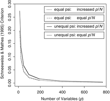
Schneeweiss and Mathes (1995) criterion (\( {\hat{\psi}}_{\max }/{\hat{d}}_{\min } \)) as a function of the number of observed variables (p) for four simulation conditions
Fig. 15.3 
Schneeweiss (1997) criterion (\( \hat{\delta}/{\hat{d}}_{\min } \)) as a function of the number of observed variables (p) for four simulation conditions
-
(2)
The average squared canonical correlations \( {\rho}^2\left(\widehat{\boldsymbol{\Lambda}},{\widehat{\boldsymbol{\Lambda}}}^{*}\right) \) increase rapidly to 1 as p increases, especially under the conditions of equal unique variances (Figs. 15.4 and 15.5). The relationship between \( {\rho}^2\left(\widehat{\boldsymbol{\Lambda}},{\widehat{\boldsymbol{\Lambda}}}^{*}\right) \) and p is displayed in Fig. 15.5 after the Fisher-z transformation of the average canonical correlation, where \( \widehat{z}=\left(1/2\right) \log \left\{\left(1+\rho \left(\widehat{\boldsymbol{\Lambda}},{\widehat{\boldsymbol{\Lambda}}}^{*}\right)\right)/\left(1-\rho \left(\widehat{\boldsymbol{\Lambda}},{\widehat{\boldsymbol{\Lambda}}}^{*}\right)\right)\right\} \) still keeps increasing as p increased from 12 to 768. The differences in the speeds with which \( \rho \left(\widehat{\boldsymbol{\Lambda}},{\widehat{\boldsymbol{\Lambda}}}^{*}\right) \) approaches 1 among the four different scenarios become clearer after the Fisher-z transformation (Fig. 15.5). Quite interestingly, the value of the Fisher-z transformed average canonical correlation and the logarithm of p are almost perfectly linearly related. For the equal unique variance case with the constant p/N condition, \( \widehat{z} = 1.002+(1.554) log(p) \) with coefficient of determination r 2 = .9999; for the equal unique variance case with the increased p/N condition, \( \widehat{z} = 1.699+(1.280) log(p) \) with r 2 = .9999; for the unequal unique variance case with the constant p/N condition, \( \widehat{z} = 1.546+(1.059) log(p) \) with r 2 = .9997; and for the unequal unique variance case with the increased p/N condition, \( \widehat{z} = 1.585+(1.034) log(p) \) with r 2 = 1.0000.
Fig. 15.4 
Average squared canonical correlation as a function of the number of observed variables (p) for four simulation conditions
Fig. 15.5 
Fisher-z transformed average canonical correlation as a function of the number of observed variables (p) for four simulation conditions
-
(3)
The average squared canonical correlation \( {\rho}^2\left(\widehat{\boldsymbol{\Lambda}},{\widehat{\boldsymbol{\Lambda}}}^{*}\right) \) increases rapidly to 1 as the ratio p/N increases, especially faster under the condition with equal unique variances (Figs. 15.6 and 15.7). Under the increased p/N condition, the value of the Fisher-z transformed average canonical correlation and the logarithm of p/N are also almost perfectly linearly related. For the equal unique variance case, \( \widehat{z}=12.080+(2.559) log\left(p/N\right) \) with r 2 = .9998, and for the unequal unique variance case, \( \widehat{z}=9.974+(2.068) log\left(p/N\right) \) with r 2 = .9999.
Fig. 15.6 
Average squared canonical correlation as a function of the ratio of number of observed variables to sample size (p/N) for the conditions with equal and unequal unique variances
Fig. 15.7 
Fisher-z transformed average canonical correlation as a function of the ratio of number of observed variables to sample size (p/N) for the conditions with equal and unequal unique variances
-
(4)
The average squared canonical correlation \( {\rho}^2\left(\widehat{\boldsymbol{\Lambda}},{\widehat{\boldsymbol{\Lambda}}}^{*}\right) \) approaches 1 as \( {\widehat{\psi}}_{\max }/{\widehat{d}}_{\min } \) approaches 0 (Figs. 15.8 and 15.9), and also as \( \widehat{\delta}/{\widehat{d}}_{\min } \) approaches 0 (Figs. 15.10 and 15.11). The speeds for \( {\rho}^2\left(\widehat{\boldsymbol{\Lambda}},{\widehat{\boldsymbol{\Lambda}}}^{*}\right) \) to approach 1 are slightly slower for the conditions with unequal unique variances than those with equal unique variances, as reflected in Figs. 15.8 and 15.10 as well as in Figs. 15.9 and 15.11. However, the speed for \( {\rho}^2\left(\widehat{\boldsymbol{\Lambda}},{\widehat{\boldsymbol{\Lambda}}}^{*}\right) \) to approach 1 under the condition with increased p/N was slower than under the condition with constant p/N case, as reflected in Figs. 15.8 and 15.9.
Fig. 15.8 
Average squared canonical correlation as a function of Schneeweiss and Mathes (1995) criterion (\( {\hat{\psi}}_{\max }/{\hat{d}}_{\min } \)) for the four simulation conditions
Fig. 15.9 
Fisher-z transformed average canonical correlation as a function of Schneeweiss and Mathes (1995) criterion (\( {\hat{\psi}}_{\max }/{\hat{d}}_{\min } \)) for the four simulation conditions
Fig. 15.10 
Average squared canonical correlation as a function of Schneeweiss (1997) criterion (\( \hat{\delta}/{\hat{d}}_{\min } \)) for the four simulation conditions
Fig. 15.11 
Fisher-z transformed average canonical correlation as a function of Schneeweiss (1997) criterion (\( \hat{\delta}/{\hat{d}}_{\min } \)) for the four simulation conditions


15.5 Discussion
Conditions for equivalence between FA and PCA loadings were derived analytically at the population level (Guttman 1956; Schneeweiss and Mathes 1995; Schneeweiss 1997). In contrast, we considered the effect of sampling errors by analyzing the sample correlation matrices with ridge FA and PCA using a simulation, with a focus on high-dimensional situations. More specifically, we investigated whether and how the average squared canonical correlation \( {\rho}^2\left(\widehat{\boldsymbol{\Lambda}},{\widehat{\boldsymbol{\Lambda}}}^{*}\right) \) approaches 1 with large p by including the conditions obtained by Guttman, Schneeweiss and Mathes, and Schneeweiss. Results indicate that the estimates of loadings by FA and PCA are rather close for all the conditions considered. For the condition with increased p/N, we tried to create a situation where p increases faster than N. In our simulation, the results under the condition with increased p/N are still similar to those under the condition with p/N being a constant. Also, the speed for the average squared canonical correlation converging to 1 under the conditions with unequal unique variances was slightly slower than that under the condition with equal unique variances. Our results indicate that the average squared correlation between the sample loading matrix from FA and that from PCA approaches 1 as p increases, while the ratio of p/N (let alone \( \sqrt{p}/\mathrm{N} \)) does not need to approach zero. Apparently, the results seem to contradict the result theoretically derived by Bai and Li (2012). Further study is needed to explain the discrepancy.
The single most interesting finding by far was that the Fisher-z transformed average canonical correlation and the logarithm of the p are almost perfectly linearly related for every condition examined in the simulation. This implies the functional relationship \( \rho \left(\widehat{\boldsymbol{\Lambda}},{\widehat{\boldsymbol{\Lambda}}}^{*}\right)={\left\{1+2/\left[{e}^{2{\widehat{\beta}}_0}{p}^{2{\widehat{\beta}}_1}-1\right]\right\}}^{-1} \) approximately holds, where \( {\widehat{\beta}}_0 \) and \( {\widehat{\beta}}_1 \) are, respectively, the intercept and slope of the simple regression line of the Fisher-z transformed average canonical correlation on the logarithm of p. Furthermore, under the increased p/N condition, the Fisher-z transformed average canonical correlation and the logarithm of ratio p/N are also almost perfectly linear related. This can be explained from the nature of our simulation design. We chose the two series of pairs (p, N) in such a way that either p/N are a constant or \( \sqrt{p}/N \) are a constant. For the latter case, let \( \sqrt{p}/N=C \). Then (1/2)log(p) = log(N) + log(C). Thus, using log(p) as a predictor is equivalent to using log(N) as a predictor, and the equation: log(p/N) = (1/2)log(p) + log(\( \sqrt{p}/N \)) = (1/2)log(p) + log(C) explains why both log(p) and log(p/N) had a linear relationship with the Fisher-z transformed average canonical correlation.
Obviously, our simulation design is far from being extensive in a sense that the ratios p/N do not include values greater than 1. More extensive simulation studies might also need to include different covariance structures, with different combinations of p and N, as well as conditions with p/N being greater than 1.
References
Anderson, T. W. (2003). An introduction to multivariate statistical analysis (3rd ed.). New York: Wiley.
Bai, J., & Li, K. (2012). Statistical analysis of factor models of high dimension. The Annals of Statistics, 40, 436–465.
Bentler, P. M., & Kano, Y. (1990). On the equivalence of factors and components. Multivariate Behavioral Research, 25, 67–74.
Buehlmann, P., & van de Geer, S. (2011). Statistics for high-dimensional data: Method, theory, and applications. Heidelberg: Springer.
Butcher, J. N., Dahlstrom, W. G., Graham, J. R., Tellegen, A., & Kaemmer, B. (1989). The Minnesota Multiphasic Personality Inventory-2 (MMPI-2): Manual for administration and scoring. Minneapolis, MN: University of Minnesota Press.
Guttman, L. (1956). “Best possible” estimates of communalities. Psychometrika, 21, 273–286.
Hastie, T., Tibshirani, R., & Friedman, J. (2009). The elements of statistical learning (2nd ed.). New York: Springer.
Hayashi, K., & Bentler, P. M. (2000). On the relations among regular, equal unique variances, and image factor analysis models. Psychometrika, 65, 59–72.
Krijnen, W. P. (2006). Convergence of estimates of unique variances in factor analysis, based on the inverse sample covariance matrix. Psychometrika, 71, 193–199.
Lawley, D. N., & Maxwell, A. E. (1971). Factor analysis as a statistical method (2nd ed.). New York: American Elsevier.
Pourahmadi, M. (2013). High-dimensional covariance estimation. New York: Wiley.
Schneeweiss, H. (1997). Factors and principal components in the near spherical case. Multivariate Behavioral Research, 32, 375–401.
Schneeweiss, H., & Mathes, H. (1995). Factor analysis and principal components. Journal of Multivariate Analysis, 55, 105–124.
Tibshirani, R. (1996). Regression shrinkage and selection via the Lasso. Journal of the Royal Statistical Society, Series B, 58, 267–288.
Velicer, W. F., & Jackson, D. N. (1990). Component analysis versus common factor analysis: Some issues in selecting an appropriate procedure. Multivariate Behavioral Research, 25, 1–28.
Yuan, K.-H. (2013, July). Ridge structural equation modeling with large p and/or small N. Paper presented at the 78th Annual Meeting of the Psychometric Society (IMPS2013), Arnhem, The Netherlands.
Yuan, K.-H., & Chan, W. (2008). Structural equation modeling with near singular covariance matrices. Computational Statistics and Data Analysis, 52, 4842–4858.
Acknowledgments
Ke-Hai Yuan's work was supported by the National Science Foundation under Grant No. SES-1461355. The authors are grateful to comments from Drs. Sy-Miin Chow and Shin-ichi Mayekawa that led to significant improvements of the article.
Author information
Authors and Affiliations
Corresponding author
Editor information
Editors and Affiliations
Rights and permissions
Copyright information
© 2015 Springer International Publishing Switzerland
About this paper
Cite this paper
Liang, L., Hayashi, K., Yuan, KH. (2015). On Closeness Between Factor Analysis and Principal Component Analysis Under High-Dimensional Conditions. In: van der Ark, L., Bolt, D., Wang, WC., Douglas, J., Chow, SM. (eds) Quantitative Psychology Research. Springer Proceedings in Mathematics & Statistics, vol 140. Springer, Cham. https://doi.org/10.1007/978-3-319-19977-1_15
Download citation
DOI: https://doi.org/10.1007/978-3-319-19977-1_15
Publisher Name: Springer, Cham
Print ISBN: 978-3-319-19976-4
Online ISBN: 978-3-319-19977-1
eBook Packages: Mathematics and StatisticsMathematics and Statistics (R0)