Mobility Models for Vehicular Communications

Abstract

The experimental evaluation of vehicular ad hoc networks (VANETs) implies elevate economic cost and organizational complexity, especially in presence of solutions that target large-scale deployments. As performance evaluation is however mandatory prior to the actual implementation of VANETs, simulation has established as the de-facto standard for the analysis of dedicated network protocols and architectures. The vehicular environment makes network simulation particularly challenging, as it requires the faithful modelling not only of the network stack, but also of all phenomena linked to road traffic dynamics and radio-frequency signal propagation in highly mobile environments. In this chapter, we will focus on the first aspect, and discuss the representation of mobility in VANET simulations. Specifically, we will present the requirements of a dependable simulation, and introduce models of the road infrastructure, of the driver’s behaviour, and of the traffic dynamics. We will also outline the evolution of simulation tools implementing such models, and provide a hands-on example of reliable vehicular mobility modelling for VANET simulation.

1 Introduction

Network solutions designed for vehicular ad hoc networks (VANETs) will play a major role in determining the level of success of vehicular communications. Given the criticality of many applications enabled by VANETs, which include road safety and traffic management services, there is a clear need for validating and testing such network solutions in the real world. However, logistic difficulties and economic issues make experimental evaluations extremely difficult to set up. Even state-of-the-art testbeds that involve car manufacturers and mobile telecommunication operators, such as sim^TD in Germany, involve a few hundred vehicles at most. Although that number may appear large, it represents less than 1 % of the total traffic in a medium-sized city.

In fact, many VANET solutions need to be evaluated over large scales (e.g., citywide) and assume nearly 100 % penetration ratios of the vehicle-to-vehicle communication technology. In order to meet these requirements, the only option is resorting to simulation. The computational resources of today’s servers allow to simulate VANETs over whole cities, and thus to evaluate even the most demanding protocols and architectures at any sensible scale. The problem shifts instead to the level of realism of the simulation, and the dominating aspect to address is that of mobility. The movement of vehicles in every day’s road traffic directly determines the position of nodes in the VANET. Therefore, the use of an unrealistic model for vehicle mobility would lead to simulation results that are biased, unreliable or even completely erroneous.

Mobility models of road traffic have been thoroughly studied in fields such as transportation research, mathematics and physics. From a viewpoint traditionally introduced by physicists, vehicular mobility can be described at three different levels, i.e., macroscopic, mesoscopic or microscopic. Figure 11.1 provides examples of these approaches in a simple scenario where the road traffic is modelled separately over three segments of a same road.

• Macroscopic models, in Fig. 11.1a represent road traffic as a hydrodynamic phenomenon, where flows of cars move along roads similarly to fluids within tubes. They aim at defining fundamental relationship among macroscopic measures such as the speed, density and in-/out-flow of vehicles. Therefore, they do not provide information about individual vehicles, but just an aggregate overview.

• Mesoscopic models, in Fig. 11.1b descend to the individual vehicle level, yet determine the speed of each car using macroscopic measures. As a result, vehicles are not independent of each other in their movement, and all drivers on the same road segment tend to, e.g., travel at the same speed.

• Microscopic models, in Fig. 11.1c treat each vehicle as an autonomous entity, and thus describe the movement of each driver independently. They allow describing complex acceleration and overtaking behaviours, which result in different speeds by cars travelling within the same road segment.

Fig. 11.1

Classification of vehicular mobility models according to their level of detail. (a) Macroscopic. (b) Mesoscopic. (c) Microscopic

The three classes of models above have advantages and disadvantages. At one end, macroscopic models only provide an aggregate and high-level view of the system, but are mathematically tractable and can be simulated at minimal computational cost. At the other end, microscopic models can be extremely detailed, but they also require significant processing power to be run at large scales. Clearly, mesoscopic models fall in between the other two classes.

In the case of VANET simulation, the choice is mandated by the fact that vehicle-to-vehicle communications have ranges in the order of hundreds of meters. This means that the precision in representing the position of each vehicle needs to be in the order of the meter or less; otherwise, inaccuracies in the mobility representation risk to bias the communication performance. As a result, the only sensible choice is that of microscopic models that consider individual vehicles and can thus output their actual location rather than an approximate one.

Within the context of microscopic modelling of vehicular mobility, several components have to be taken into account in order to obtain a realistic representation of road traffic.

First, one needs a faithful description of the road infrastructure. The term is to be intended in its largest acceptation, i.e., not limited to a graph-like model of the road layout, but including, e.g., speed limits, one-way constraints, traffic lights at intersections and their temporization, stop and yield signs, roundabouts, overpasses, highways ramps, etc. We discuss the representation of the road infrastructure in Sect. 11.2.

Second, the microscopic behaviour of each driver must be modelled in an accurate way. The acceleration and speed of each vehicle must be the result of its interactions with surrounding cars and with the road signalization. Models of the driver’s behaviour used in the networking literature are presented in Sect. 11.3.

Third, traffic flows of individual vehicles over the road topology must be properly described. In other words, the trip of each car is to be detailed, in terms of its origin location, its destination, and the time at which the trip starts. This maps to the definition of a so-called travel demand. Moreover, once trips are decided, the precise route taken by drivers needs to be selected, via apt traffic assignment models. Modelling of traffic flows in works on VANETs is introduced in Sect. 11.4.

These three components have been progressively included in tools dedicated to the simulation of microscopic vehicular mobility for networking purposes. We briefly review the evolution of such tools in Sect. 11.5, so as to provide the reader with an overview of the dramatic improvements that have occurred in VANET simulation over the last decade.

Finally, in Sect. 11.6, we provide a thorough description of the generation process of one specific state-of-the-art dataset of vehicular mobility. This hands-on example brings together different models and tools discussed in the previous sections of the chapter, and allows us to stress the challenges encountered during the creation of a large-scale road traffic trace.

2 Modeling Road Topologies

The road topology is an important factor accounting for mobility in simulations, since the topology constrains cars’ movements, see Cavin et al. [6]. For MANETs, the random waypoint model (RWP) [46] is by far the most popular mobility model. However, in vehicular networks, nodes (vehicles) do not move independently of each other but they move according to a well-established vehicular traffic models, so the results for MANETs cannot be directly applicable. Moreover, vehicles can only move along streets, prompting the need for a road topology model.

Roughly described, an urban topology is a graph where vertices and edges represent, respectively, junction and road elements. Simulated road topologies can be generated ad hoc by users, randomly by applications, or obtained from real roadmap databases. Using complex layouts implies more computational time, but the results obtained are closer to reality.

The two most typical topologies used are: the highway scenarios (the simplest layout, basically a straight line without junctions) and the Manhattan-style street grids (with streets arranged orthogonally). For example, Huang et al. [18] studied taxi behaviour modelling the city as a Manhattan style grid with a uniform block size across the simulation area. All streets were assumed to be two-way, with one lane in each direction; taxi movements were constrained by these lanes. Figure 11.2 shows two examples of synthetic topologies: (a) used defined, and (b) Manhattan-based, respectively.

Fig. 11.2

Examples of different roadmap topologies: (a) user defined, and (b) Manhattan

These approaches are simple and easy to implement in a simulator. When used, results can give some information about the general performance trends of the different algorithms studied. However, a more realistic layout should be used to ensure that the results are closer to reality.

As proposed by Jardosh et al. [20], a possible solution to randomly generate graphs on a particular simulation area is Voronoi tessellations. With this approach we start by distributing points, representing obstacles (e.g., buildings), over the simulation area. We then draw the Voronoi domains, where the Voronoi edges represent roads and intersections running around obstacles. This way we obtain a planar graph representing a set of urban roads, intersections and obstacles. Figure 11.3 depicts two random Voronoi maps: (a) with uniform density of streets, and (b) clustered density of streets.

Fig. 11.3

Examples of different roadmap topologies: (a) Voronoi uniform, and (b) Voronoi clustered

Although being an interesting improvement, these graphs lack realism too. Indeed, the distribution of obstacles should be fitted to match specific urban configurations. For instance, dense areas such as city centres have a larger number of obstacles, which in turn increases the number of Voronoi domains. By looking at topological maps, we can see that the density of obstacles is higher in the presence of points of interest. To address these issues, generating clusters of obstacles with different densities is required.

Saha and Johnson [36] modelled vehicular traffic as the random movement of vehicles over real road topologies extracted from the maps of the US Census Bureau TIGER database. In that work, the vehicles selected one point over the graph as their destination and computed the shortest path to get there. The edges sequence is obtained weighting the cost of traveling on each road at its speed limit, including the traffic congestion. Currently, similar approaches are being used by using maps coming from other sources, like OpenStreeMap.org (see Fig. 11.4.)

Fig. 11.4

Examples of different roadmap topologies: (a) TIGER database, and (b) openstreetmap.org

3 Modeling Driver’s Behaviour

Major studies have been undertaken in order to develop mathematical models reflecting a realistic physical effect. Fiore et al. [12] wrote a complete survey of models falling into this category. According to Fiore’s classification, drivers behaviour can be classified in to five groups: (1) Stochastic models wrapping all models containing purely random motions, (2) Traffic Stream models looking at vehicular mobility as hydrodynamic phenomenon, (3) Car Following models, where the behaviour of each driver is modelled according to vehicles ahead, (4) Queue models, which model roads as FIFO queues and cars as clients, and (5) Behavioural models, where each movement is determined by behavioural rules such as social influences. In the following subsections we will give the most relevant example of mobility model for each sub-category.

3.1 Stochastic Models

The Manhattan mobility model [5] is the most widely used example of a Stochastic model which uses a grid road topology (see Fig. 11.2b). The Manhattan model employs a probabilistic approach in the selection of node movements, since, at each intersection, a vehicle chooses to keep moving in the same direction with a 50 % probability, and to turn left or right with a 25 % probability in each case. Vehicles move over the grid with constant speed. The car interaction rules usually employed in the Manhattan model are too simple and do not reproduce a realistic driver behaviour.

3.2 Traffic Stream Models

The Fluid Traffic Motion (FTM) [37] is an example of a Traffic Stream model which accounts for the presence of nearby vehicles when calculating the speed of a car. This model describes car mobility on single lanes, but does not consider the case in which multiple vehicular flows have to interact, as in the presence of intersections.

The FTM describes the speed as a monotonically decreasing function of the vehicular density, forcing a lower bound on speed when the traffic congestion reaches a critical state by means of the following equation:

$$\displaystyle\begin{array}{rcl} s = \mathrm{max}\left [s_{\mathrm{min}},s_{\mathrm{max}}\left (1 - \frac{k} {k_{\mathrm{jam}}}\right )\right ]& &{}\end{array}$$

(11.1)

where s is the output speed, s _min and s _max are the minimum and maximum speed, respectively, k _jam is the vehicular density for which a traffic jam is detected, and k is the current vehicular density of the road where the node is, whose speed is being computed, is moving on. This last parameter is given by $k = n/l$, where n is the number of cars on the road and l is the length of the road segment itself.

According to this model, cars traveling on very crowded and/or very short streets are forced to slow down, possibly to the minimum speed, if the vehicular density is found to be higher than or equal to the traffic jam density. On the other hand, as less congested and/or longer roads are encountered, the speed of cars is increased towards the maximum speed value. Thus, the Fluid Traffic Model describes traffic congestion scenarios, but still cannot recreate queuing situations, nor can it correctly manage car behaviour in the presence of road intersections. Moreover, no acceleration is considered and it can happen that a very fast vehicle enters a short/congested edge, suddenly changing its speed to a very low value, which is definitely a very unrealistic situation.

3.3 Car Following Models

The Krauss Model [26] falls into the Car Following Model subcategory. It takes four input variables (the maximum velocity v _max, the maximum acceleration a, the maximum deceleration b, and the noise η that introduces stochastic behavior to the model), discretizes the time with step Δ t, and is defined by the following set of equations:

$$\displaystyle\begin{array}{rcl} \upsilon _{i}^{\mathrm{safe}}(t +\varDelta t) =\upsilon _{ i+1}(t) + \frac{\varDelta x_{i}(t) -\upsilon _{i+1}(t)\tau } {(\upsilon _{i}(t) +\upsilon _{i+1}(t))/2b+\tau }& &{}\end{array}$$

(11.2)

$$\displaystyle\begin{array}{rcl} \upsilon _{i}^{\mathrm{desired}}(t +\varDelta t) = \mathrm{min}\left [\upsilon _{\mathrm{ max}},\upsilon _{i}(t) + a\varDelta t,\upsilon _{i}^{\mathrm{safe}}(t +\varDelta t)\right ]& &{}\end{array}$$

(11.3)

$$\displaystyle\begin{array}{rcl} \upsilon _{i}(t +\varDelta t) = \mathrm{max}\left [0,\upsilon _{i}^{\mathrm{desired}}(t +\varDelta t) -\epsilon \: a\:\varDelta t\:\eta \right ]& &{}\end{array}$$

(11.4)

Equation (11.2) computes the speed of vehicle i required to maintain a safety distance from its leading vehicle. The reaction time of the driver is represented by the time τ. Equation (11.3) determines the new desired speed for vehicle i, which is equal to the current speed plus the increment determined by the uniform acceleration, with upper bounds represented by the maximum and safe speeds. Equation (11.4) finally determines the speed of the following vehicle, by adding some randomness, in the measure of a maximum percentage ε of the highest achievable speed increment a Δ t (η is a random variable uniformly distributed in [0, 1]).

Another interesting example was the Intelligent Driver model, presented by Treiber et al. [41]. Such model characterizes drivers behaviour depending on their front vehicle. The instantaneous acceleration of a vehicle is computed according to the following equations:

$$\displaystyle\begin{array}{rcl} \frac{\mathit{dv}} {\mathit{dt}} = a\left [1 - \frac{\upsilon } {\upsilon _{0}}^{4} -\frac{s^{{\ast}}} {s} ^{2}\right ]& &{}\end{array}$$

(11.5)

$$\displaystyle\begin{array}{rcl} s^{{\ast}} = s_{ 0} +\upsilon T + \frac{\upsilon \varDelta \upsilon } {2\sqrt{\mathit{ab}}}& &{}\end{array}$$

(11.6)

In Eq. (11.5), υ is the current speed of the vehicle, υ ₀ is the desired velocity, s is the distance from preceding vehicle, and s ^∗ is the so-called desired dynamical distance. This last parameter is computed as shown in Eq. (11.6), and is a function of the minimum bumper-to-bumper distance s ₀, the minimum safe time headway T, the speed difference with respect to front vehicle velocity Δ υ, and the maximum acceleration and deceleration values a and b.

When combined, these formulae give the instantaneous acceleration of the car, divided into a “desired” acceleration [υ∕υ ₀ ⁴] on a free road, and braking decelerations induced by the preceding vehicle [s ^∗∕s ²]. By smoothly varying the instantaneous acceleration, the IDM can realistically mimic car-to-car interactions on a single-lane and straight road. Interesting real-world situations, such as queuing of vehicles behind a slow car, or speed reduction in presence of congested traffic can be reproduced. However, this model alone is not yet sufficient to obtain a realistic vehicular mobility model for urban environments.

Two different extensions were proposed to complete the model: (1) IDM with Intersection Management (IDM-IM), which adds intersection-handling capabilities to the behaviour of vehicles driven by the IDM, and (2) IDM with Lane Changing (IDM-LC), which extends the IDM-IM model with the possibility for vehicles to change lane and overtake each others, taking advantage of the multi-lane capability of the macro-mobility description.

3.4 Queue Models

Queue models were introduced in the vehicular traffic field by Gawron [14]. According to the queue paradigm, each road is modelled as a FIFO queue, and each vehicle as a queue client. Each road queue k is characterized by its length l ^k and a maximum flow q ^k_max , determined by the number of lanes. Every time a vehicle enters a road, a travel time is computed, depending on the desired free flow speed of the driver v _max, on the number of vehicles on the road n ^k and the road length.

The car is then queued in the priority queue of the road, according to the travel time calculated before. At every time step, vehicles whose travel time has expired can be removed from the head of the queue and inserted into the queue representing the next road in their trip. However, when multiple choices are available to exit a road, an intermediate step is necessary, and first-in-first-out queues are added for each outgoing flow. In that case, vehicles at the head of the priority queue are moved to one of the FIFO queues, depending on their destination.

The FIFO queues have a finite capacity, meaning that only a certain number of vehicles per second can access them. Since the movement from one road to another is constrained by the capacity of such next road, a vehicle at the head of an output queue can join the following queue only if there is space on the following road.

The capacity of a road is easily modelled as $c^{k} = \frac{n^{k}q_{\mathrm{ max}}^{k}} {x_{\mathrm{min}}}$, where x _min is the distance between the front of two adjacent vehicles in jam conditions. Thus, if the new road has c ^k cars already queued, it will not accept further vehicles, and drivers willing to enter the road will have to wait until a spot is freed.

It was shown [14] that even a simple expression of travel time l ^k∕v _max, which neglects the effect of vehicular density on the speed, leads to very good approximations of results obtained with much more complex microscopic mobility models.

Since queue models describe the movement of each vehicle in an independent way, but also with a minimal level of detail, they fall into an intermediate category with respect to macroscopic and microscopic descriptions, which can be referred to as mesoscopic. Queues models have very low computational cost, because they update the status of a vehicle only when a vehicle enters a new priority or FIFO queue. This allows to model very large road topologies, up to hundreds of thousands of vehicles. The drawback is the reduced realism of the outcome, which is less precise than that obtained with other models (e.g., queue models do not reproduce shockwaves caused by periodic perturbations, a common phenomenon in vehicular traffic).

3.5 Behavioural Models

Legendre et al. [27] introduced a novel approach to the problem of modelling human mobility, which can be applied to vehicular traffic as well. The approach was called behavioural modelling, and is borrowed from the fields of biological physics and artificial intelligence. The key idea is that every movement is determined by behavioural rules, which are imposed by social influences, rational decisions or actions following a stimulus-reaction process. These rules can be modelled as attractive or repulsive forces. In the case of vehicular mobility, the next intersection towards the trip destination wields an attractive force on the vehicle, whereas other vehicles or obstacles in general exert a repulsive force on it. The result from the composition of these forces determines the acceleration vector driving the car movement. This model is especially expensive under the computational point of view, as every movement requires the elaboration and composition of multiple inter-object forces.

4 Modeling Traffic Dynamics

Due to the complexity of modelling vehicular mobility, only few synthetic models are able to come close to a realistic modelling of motion patterns. A different approach could also be followed. Instead of developing complex synthetic models and then calibrating them using mobility traces or surveys, time could be saved by directly extracting generic mobility patterns from movement traces.

Such approach became increasingly popular as mobility traces started to be gathered through the various measurement campaigns launched by activities such as: (1) the project developed in conjunction with the Fleetnet Project—Internet on the Road [13] and the NOW—Network on Wheels Project [33], which is based on traces measured by Daimler AG on a highway section, (2) the UMass DieselNet Project [43], created by the University of Massachusetts, which provides mobility traces of a bus system in the city of Amherst, MA, USA, and (3) the Cabspotting Project [4] which equipped all taxi vehicles in the San Francisco Bay Area and provides a live visualization of the complete taxi system.

The most difficult part of this approach is to extrapolate patterns not observed directly by traces. Complex mathematical models are required to predict mobility patterns, but their limitations are mainly linked to the class of the measurement campaign. For instance, if motion traces have been gathered for bus systems, an extrapolated model cannot be applied to the traffic of personal vehicles. Another limitation for the creation of trace-based vehicular mobility models is the limited availability of vehicular traces.

Surveys are also an important source of macroscopic mobility information. The major large scale surveys are provided by the US Department of Labor (DOL),¹ which gathered extensive statistics of US workers’ behaviours, spanning from the commuting time or lunch time, to traveling distance or preferred lunch types. By including such kind of statistics into a mobility model, one is able to develop a generic mobility model able to reproduce the pseudo-random or deterministic behaviour observed in the real urban traffic.

Mobility simulators implementing survey-based models simulate arrival times at work, lunch time, breaks/errands, pedestrian dynamics (e.g., realistic speed-distance relationship and passing dynamics), and workday time-use such as meeting size, frequency, and duration. Vehicle traffic is derived from vehicle traffic data collected by state and local governments and models vehicle dynamics and diurnal street usage.

The UDel Models For Simulation of Urban Mobile Wireless Networks [42] typically falls into the survey-based models category. Its mobility simulator is based on surveys coming from various areas. It includes: (1) time-use studies performed by the US Department of Labor and Statistics, (2) time-use studies by the business research community, (3) pedestrians and vehicle mobility studies by the urban planning and traffic engineering communities. Vehicle traffic is derived from vehicle traffic data collected by state and local governments and models vehicle dynamics and diurnal street usage.

Another Survey-based model is the Agenda-based [47] mobility model, which combines both social activities and geographic movements. The movement of each node is based on an individual agenda, which includes all kinds of activities in a specific day. Data from the US National Household Travel Survey has been used to obtain activity distributions, occupation distributions and dwell time distributions.

A complex and computationally demanding vehicular mobility model was proposed by the ETH Laboratory for Software Technology [10], which generates public and private vehicular traffic over real regional roadmaps of Switzerland with a high level of realism within a period of 24 h. The model is calibrated using data from census and other local or national mobility surveys or statistics.

The limitation of the survey-based approaches is that survey or statistical data are only able to provide a coarse grain mobility characterization, modelling global mobility patterns instead of precise movements. Yet, it has the advantage of being able to represent a particular mobility that would be too complex to model by mathematical equations.

5 Evolution of Software Tools for Mobility Modelling

The generation of synthetic traces of road traffic is an important requirement in transportation engineering, and a long-studied topic in transportation research. Simulated traces are required in order to understand the weaknesses of transportation systems, and to design and assess potential solutions to the same. However, in many cases, engineering new road infrastructures and devising apt road traffic policies only require a characterization of macroscopic traffic densities and flows. For that objective, simulators focused on traffic assignment, such as MatSim,² are sufficient. These tools yield however low detail in the representation of the precise movement of each vehicle, which is instead needed for the evaluation of network solution involving communication-enabled cars. In fact, there exist several fine-grained simulators developed for transportation planning; however, they are typically commercial, including TSIS-CORSIM,³ Paramics,⁴ and VISSIM.⁵ Moreover, these tools have a steep learning curve, which represents a major obstacle for many networking researchers who are not willing to spend a significant amount of time on pure road traffic modeling aspects.

The need for high-detail, freely available, and easy-to-use software led at first the networking community to start developing its own vehicular mobility simulation frameworks. Initially, reuse of well-known stochastic models commonly employed in mobile ad hoc network (MANET) scenarios appeared as the easiest choice. However, it was soon clear that the likes of Random Waypoint and Random Direction could not be representative of real-world vehicular mobility.

Thus, early attempts at simulating a more realistic movement of vehicles approximated the road topology with regular grids, and the movement of vehicles with constant-speed random trips constrained over these grids. That is the case, e.g., of the tools introduced by Davies [8].

Improvements to the representation of the street layout consisted at first in the possibility of manually defining the road topology. In particular, the CanuMobiSim framework by Tian et al. [39] allowed users to draw graphs where vertices mapped to road intersections and edges to streets joining them. In a second moment, real-world road networks started to be considered, mainly thanks to the public availability of databases such as the US Census TIGER in North America or Ertico GDF in Europe. In particular, Saha and Johnson [36] were the first to employ realistic maps for the study of vehicular networks. However, random trips at constant speed—even if constrained to a realistic road layout—still led to questionable conclusions, e.g., that vehicular mobility could be approximated with unconstrained and fully random movements.

Aware of these problems, the networking research community started to include in their vehicular mobility simulation frameworks more credible speed models. Seminal work was carried out by Bai et al. [1], who introduced the IMPORTANT framework. The latter features an original speed model, named the freeway model, based on probabilistic acceleration and bounded speed in order to force each driver to avoid contact with the vehicle ahead. In fact, the freeway model and its extensions were still far from being realistic. Fiore and Härri [11] demonstrated how these models could not pass basic validation tests developed by the transportation research community. The same authors also showed that driver’s behaviour models introduced in transportation research (discussed in detail in Sect. 11.3) proved to be much more reliable—and that such a different level of realism had a significant impact on the connectivity properties of the vehicular network.

As a consequence, the networking community begun developing frameworks that integrated, e.g., car-following or cellular automata models borrowed from the rich literature in transportation research. Commonly employed models include those by Treiber et al. [41], Krauss et al. [26], Nagel and Schreckenberg [31]. This resulted in public availability of a number of tools specifically dedicated to the simulation of vehicular mobility for network studies, such as FreeSim by Miller and Horowitz [30], GrooveNet by Mangharam et al. [28], MoVes by Bononi et al.[3], and the City Model by Jaap et al. [19].

Such frameworks did not yet allow to account for overtakings, in- and out-flows of vehicles through highway ramps, stop signs or traffic lights at road intersection. All these features are mandatory in complex road traffic simulations of both highway and urban environments. Therefore, in order to include them in the generation process, new tools appeared that also implemented lane changing and intersection management models. The latter were again mostly borrowed from the transportation research literature: common examples are those of the models proposed by Krauss [25], Treiber and Helbing [40], Nagel et al. [32]. Among the most popular vehicular mobility simulation tools that also include such models, we can mention STRAW by Choffnes and Bustamante [7], GMSF by Baumann et al. [2], Udel Models by Kim et al. [21], CityMob by Martinez et al. [29], VanetMobiSim by Härri et al. [16], and SUMO by Krajzewicz et al. [24].

More recently, the most advanced road traffic generators have become part of federated tools that allow run-time interoperability between mobility and network simulators. These tools thus allow to perform vehicular networking simulations that are especially flexible and accurate. On the one hand, using two separate and dedicated tools to reproduce the vehicular mobility as well as the network channel and protocol stack guarantees the accuracy of the representation of each aspect. On the other hand, run-time interaction among the two tools allows (1) the road traffic conditions to trigger network protocol (and overlying service) operation, and (2) the messages received by connected vehicles to influence drivers’ behaviour. Overall, federated frameworks represent the current state of the art in the simulation of vehicular networks. Examples of such tools include TraNS by Piorkowski et al. [34], iTetris by Krajzewicz et al. [23], and Veins by Sommer et al. [38].

For a comprehensive discussion of most of the tools mentioned above, we refer the reader to the very complete survey by Haerri et al. [15]. The current state-of-the-art federated tools we mentioned at the end of the discussion will instead be presented in detail in Chap. 13

6 A Hands-on Example: Generating an Urban-Scale Road Traffic Dataset

In this section, we present how the tools introduced previously in this chapter can be brought together so as to generate a comprehensive road traffic dataset, specifically designed for networking studies. The specific dataset we present is a contribution to the TAPASCologne initiative⁶ of the Institute of Transportation Systems at the German Aerospace Center (ITS-DLR), which aims at reproducing microscopic car traffic in the greater urban area of the city of Cologne, Germany, with the highest level of realism possible. The detailed description of the process is intended to be useful to researchers who are willing to replicate it and produce their own synthetic traces of vehicular mobility.

As a first step, we detail the data sources employed to generate the dataset, which are listed next.

• Road infrastructure. The first source is a detailed description of the road infrastructure. This includes not only the street layout, but also information on the road type and capacity, on per-road speed limits, on intersection signalization, and on the presence of specific structures such as ramps, roundabouts or overpasses. For the dataset under consideration, the road infrastructure data of the Cologne urban area is obtained from the OpenStreetMap (OSM) database.⁷ The OSM project provides freely exportable maps of cities worldwide, which are contributed and updated by a vast user community. Maps include most of the needed information, as generated and validated by means of satellite imagery and GPS traces, and it is commonly regarded as the highest-quality road data publicly available today. The OSM data is filtered with the Osmosis tool⁸ so as to extract the road topology information for an area of approximately 400 km² centred in the urban agglomeration of Cologne, and including around 4,500 km of roads. The Java OSM Editor⁹ is used to repair the OSM data and make it compatible with the microscopic mobility simulator, as later detailed in this section. Considering open-source data only, OSM represent the de-facto standard choice to infer the road infrastructure needed for the generation of synthetic microscopic road traffic traces.

• Microscopic vehicular mobility. The microscopic mobility of vehicles is simulated with the Simulation of Urban Mobility (SUMO) software.¹⁰ SUMO is an open-source, space-continuous, discrete-time traffic simulator developed by the German Aerospace Center (DLR), capable of accurately modelling the behaviour of individual drivers, accounting for car-to-car and car-to-road signalization interactions. More precisely, SUMO can import road maps and information on traffic lights, roundabouts, stop and yield signs from multiple formats, including OSM. The microscopic mobility models implemented by SUMO are Krauss’ car-following model [26] and Krajzewicz’s lane-changing model [22], that respectively regulate each driver’s acceleration and overtaking decisions, by taking into account a number of factors, such as the distance to the leading vehicle, the traveling speed, and the acceleration and deceleration profiles. These models have been long validated by the transportation research community, a fact that, jointly with the high scalability of the simulator, makes of SUMO the most complete and reliable among today’s open-source microscopic vehicular mobility generators. The version we employed for the dataset generation is 12.3, but the simulator has further evolved then since. We refer the reader to Chap. 13 for a detailed introduction to SUMO.

• Travel demand. The travel demand information on the macroscopic traffic flows across the Cologne urban area is inferred via the Travel and Activity PAtterns Simulation (TAPAS) methodology [45]. This technique generates an origin-destination matrix of the population mobility by exploiting information on (1) the population itself, i.e., home locations and socio-demographic characteristics, (2) the points of interests in the urban area, i.e., places where work and free-time activities take place, and (3) the time use patterns, i.e., habits of the local residents in organizing their daily schedule [17]. Within the context of the TAPASCologne project, TAPAS is applied to real-world data collected in the Cologne region by the German Federal Statistical Office, including 30,700 daily activity reports from more than 7,000 households [9, 35]. The resulting origin-destination matrix faithfully mimics the daily movements of inhabitants of the area over 24 h, for a total of 1.2 million individual trips. Among the data sources needed for to complete the generation process, the travel demand is without doubt that most difficult to retrieve. Within that context, the TAPASCologne origin-destination matrix is, up to now, the only realistic traffic demand dataset of a large urban region that has been disclosed.

• Traffic assignment. The actual assignment of the vehicular traffic flows described by the TAPASCologne origin-destination matrix over the road topology is performed by means of Gawron’s algorithm [14]. This traffic assignment technique computes the fastest route for each vehicle, and then assigns to each road segment a cost reflecting the intensity of traffic over it. By iteratively moving part of the traffic to alternate, less congested paths, and recomputing the road costs, the scheme finally achieves a so-called user equilibrium. Additionally, since the intensity of the traffic demand varies over a day, the traffic assignment model must also be able to adapt to the time-varying traffic conditions. Indeed, Gawron’s algorithm satisfies such a requirement, thus attaining a so-called dynamic user equilibrium. Gawron’s is one of the most popular traffic assignment techniques developed within the transportation research community, and allows to reach a road capacity utilization close to reality and significantly higher than that obtained with, e.g., a standard weighted Dijkstra algorithm. Moreover, an implementation is embedded in SUMO, which eases its adoption by the research community.

The individual components presented above are combined as depicted in Fig. 11.5 in order to generate the vehicular mobility dataset. First, the information contained in the TAPASCologne origin-destination matrix are used to identify the boundaries of the exact simulation region, extract the associated map from OSM and filter it so as to remove unneeded content that does not concern the road layout. Then the OSM map is converted to a format readable by SUMO, and fed to the microscopic mobility simulator. The TAPASCologne origin-destination matrix is also used as an input to Gawron’s algorithm, which, in turn, determines an initial traffic assignment and provides it to SUMO. At this point, a first vehicular mobility simulation can be started with SUMO. Once the first run finished, a feedback on the resulting traffic density over the road topology is sent back to Gawron’s algorithm. Based on this new information, a new traffic assignment is computed, and a second SUMO simulation is run. The process is iterated until we obtain a traffic assignment that allows to sustain the whole volume of the traffic demand, and further iterations do not bring advantage in terms of the aggregate travel time of all vehicles.

Fig. 11.5

Simulation workflow (figure appeared in Uppoor et al. [44])

Unfortunately, making all of the previous components work together is not a straight procedure. Figure 11.6a shows the result obtained by simply running the SUMO simulation with the data sources made available by OSM and TAPASCologne. The plot details the temporal evolution of the number of vehicles that (1) are traveling on the road topology, (2) have successfully ended their trip by reaching their destination, (3) are waiting to enter the road topology due to excessive congestion at entry points. The latter is an undesirable simulation artefact, identifying situations where the road topology cannot accommodate all the travel demand. The number of traveling vehicles present in the simulation rapidly grows up to exceed a hundred thousands units, a figure completely unrealistic for a city the size of Cologne. Additionally, such a number does not tend to decrease as one could expect once the morning traffic peak ends; instead, it keeps growing indefinitely. We also observe that the number of vehicles that end their trip grows very slowly over time, as only a very small fraction of the cars that are present on the road topology can reach their destination. Finally, the number of vehicles that are waiting to enter the road topology, which we would like to stay as close as possible to zero, grows to hundreds of thousands of units.

Fig. 11.6

Original TAPASCologne dataset. (a) Traffic features over time. (b) Snapshot of the traffic status at 7:00 a.m., in a 400 km² region centred on the city of Cologne (figure appeared in Uppoor et al. [44])

These results are clear symptoms of how the road topology cannot sustain the volume of cars injected according to the traffic demand model. Indeed, when looking at a snapshot of the car traffic in the region, it is evident how the simulation quickly reduces to a huge traffic jam. As an example, Fig. 11.6b depicts the map of the road traffic at 7:00 a.m., with each dot representing one vehicle. The road topology presents a very high number of dots gathered together along major arteries, representing cars stuck in heavily congested traffic. Next, we discuss the reasons for such a result, and present solutions to them.

6.1 Repairing the Dataset

The poor outcome of the road traffic simulation is the result of the combination of a number of undesirable effects emerging when the different tools discussed before are coupled into a single generation process, as follows.

• Over-comprehensive and bursty traffic demand. The original TAPASCologne origin-destination matrix yields the traffic demand volume depicted in Fig. 11.7a, which shows the number of vehicles injected in the whole road network every second. There, we identified and fixed three major problems. First, the demand is not limited to vehicular traffic, but also includes information on the daily trips of all Cologne inhabitants. We thus pruned it, considering that around 50 % of the overall trips are performed by drivers in the region [17, Fig. 4]. Second, the demand presents sudden peaks, unrealistic given that the traffic is aggregated over a very large area. We smoothed down the original matrix, by introducing a random jitter in departure times that allows to remove the injection bursts, yet retaining the demand properties over larger time scales. Third, the demand only includes trips starting or ending within the 400 km² simulated region. We employed historic data from the Nordrhein–Westfalen Ministry of Transport¹¹ to introduce the missing highway traffic in the demand.

  Fig. 11.7

  

  Original data sources. (a) Volume of traffic injected in the road network between 6:00 a.m. and 12:00 p.m., according to the originalTAPASCologne origin-destination matrix. (b) Example of wrong restriction in OSM. (c) Example of continuous restriction in OSM (figure appeared in Uppoor et al. [44])

• Inconsistent road information. Although very complete from a topological viewpoint, the OSM map embeds information at times inconsistent with respect to reality. The impact of such inconsistencies, albeit negligible on most of the usages of OSM, can be dramatic for the simulation of vehicular mobility. A first type of inconsistency is represented by wrong traffic movement restrictions enforced on some road segment, e.g., in Fig. 11.7b: there, a restriction is present that prevents cars from turning left. At times, wrong restrictions of this kind are present in the OSM data, forcing vehicles to perform long detours or to wait indefinitely for a possibility to turn and continue their journey. Visual inspection against Google Street View allowed us to fix approximately one thousand erroneous restrictions in the area under study. A second type of inconsistency is that of correct movement restrictions being enforced on the whole road extent, whereas they only apply to road portions. Figure 11.7c portrays an example where two one-way roads cross each other. In the real world, the roads pass one over the other, and vehicles traveling on one road can join the other by means of the slanting relief route. In the OSM road representation, the horizontal road is represented by a sequence of segments all featuring an only-straight traffic restriction. This prevents vehicles from considering the overpass as an intersection, but also from taking the relief route. Such situations occur in most of the interchange nodes among high-speed roads. We solved the problem by separating the segments of approximately 800 roads, to which we assigned correct restrictions.

• Flawed road topology conversion. The OSM road information is natively imported by SUMO through an automated conversion process that proves not to be error-free. First, attributes with multiple values are considered as incorrect by the converter, as in Fig. 11.8a, and the associated roads are removed from the SUMO topology, as in Fig. 11.8d. Second OSM rendering of complex intersections is unfit for direct conversion to SUMO street layout. As an example, the crossroad in Fig. 11.8b is modeled in OSM as a sequence of multiple junction, each regulated by a different traffic light. Conversion of the latter within SUMO results in an exceedingly intricate intersection, where vehicles get stuck and rapidly form a permanent traffic jam, Fig. 11.8e. Third, the OSM data contains at times traffic lights that are not present in the real world; moreover, the SUMO converter employs by default a technique to deploy additional traffic lights over the street layout. We corrected the OSM data by making all attributes compatible with the SUMO converter, by joining road segment links that refer to the same physical intersection, and by removing unrealistic traffic lights from the OSM data.

  Fig. 11.8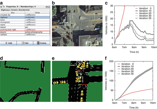

  

  Original data sources. (a, d) Example of unrecognized information ignored during map conversion. (b, e) Example of topological information unfitness during map conversion. (c, f) Traffic evolution over multiple iterations of the assignment algorithm (figure appeared in [44])

• Simplistic default traffic assignment. Running the microscopic mobility simulation, with the corrected travel demand and road topology still results in widespread road traffic congestion. The reason lies in the traffic assignment, i.e., the way drivers choose the route to reach their intended destination. By employing Gawron’s traffic assignment algorithm, a dynamic user equilibrium is reached after 35 iterations. Figure 11.8c shows the evolution of the number of vehicles traveling at the same time over the road topology, which tends to explode during the first iterations, but is reduced already at the 10th iteration. Figure 11.8f confirms that iterations increase the number of vehicles that can successfully reach their destination.

6.2 Final Dataset

The resulting dataset comprises more than 700,000 car trips in the Cologne larger metropolitan area, over a period of 24 h. The simulated traffic mimics the normal daily road activity in the region, as the fixed road topology can accommodate the updated traffic demand and assignment. Evidences of the correct behaviour of the simulated mobility are given in Fig. 11.9a. By comparing it to the equivalent plot before repair, in Fig. 11.6a, it is clear that the number of traveling cars now follows the traffic demand, with peaks during the morning (from 7:00 a.m. to 9:00 a.m.) and afternoon (from 4:30 p.m. to 6:00 p.m.) rush hours. An approximate maximum of 15,000 vehicles travel at the same time over the road topology, at around 8:00 a.m. Real-world behaviours, such as very low traffic at night and a lower traffic peak at around noon, can also be observed. Also, the number of ended trips now grows over time, as more and more drivers reach their destinations, and the number of vehicles waiting to enter the simulation is reduced to values close to zero. As a result, the road traffic at 7:00 a.m., in Fig. 11.9b, looks significantly better than the original one, in Fig. 11.6b. Indeed, large portions of the urban road layout present a sparse density of points, indicating fluid traffic conditions. The traffic appears only congested in the city centre, where higher concentrations of dots are visible. However, this represents a normal condition in Cologne at that time, and, moreover, the congestion level is much lower than that recorded over vast regions in Fig. 11.6b.

Fig. 11.9

Original TAPASCologne dataset. (a) Traffic features over time. (b) Snapshot of the traffic status at 7:00 a.m., in a 400 km² region centred on the city of Cologne (figure appeared in Uppoor et al. [44])

7 Future Perspective

The modelling of mobility is still an active area and various aspects must still be considered. The final goal is finding the best approximation of real mobility pattern to achieve that modelling or simulation results of VANETs scenario are as close as possible to reality. With this aim various factors are to be introduced and represented in the future solution.

First of all, the structure of the roads layout and the streets configuration should provide the possibility to represent different categories (rural, highway, etc.), multiple lanes, and different maximum velocities. Also, the road crossing average or density should be considered. For certain types of applications, reaching a higher level of detail, thus including possible obstacles on the road, like bumpers, could result to be very useful.

Moreover, the driving manner of users should be considered, like the way they decelerate or accelerate or brake, since it impacts on the interaction with the environments. Also, regarding the chosen route, different drivers may have different needs, which affect their route selection. Therefore, the mobility model should control the interactions between vehicles, especially in situations like traffic jam or overtaking. The modelling of the behaviour at the intersections should also be improved. The driver behaves differently whether he finds a stop signs, a yield sign, or a traffic light.

The type and characteristics of the vehicle should be modelled. It is not the same to consider a truck on a rural road than on a highway. Moreover, acceleration, deceleration and speed capabilities of a car or a truck are different. Accounting for these characteristics alters the traffic generation engine when modelling realistic vehicular motions.

The so-called Attraction points should be included in a path like time patterns. The final destinations of many road trips are typically shared among various users, likewise the initial locations, called repulsion points (e.g. main entrance avenues). Traffic density strongly depends on the time of the day, the day of the week and the period in the year. Traffic is not the same on a summer Sunday morning than a Monday morning in February. Driver can even change their trip preferences depending of the time and date.

Finally, random and external events should be considered to include the influence of accidents, temporary road works, or real-time knowledge of the traffic status on the motion constraints and the traffic generator blocks.

A vehicular mobility model will be more precise as the number of factors it includes will increase. Parameters defining the different major building blocks such as topological maps, car generation engine, or driver behaviour engine cannot be randomly chosen but must reflect realistic configurations. Therefore, due to the large complexity to obtain such kind of information, the research community took more simplistic assumptions and neglected several factors. Currently most models available include a topological map, or at least a graph, as motion constraints. However, they do not include speed constraints or more generally attraction or repulsion points. The car generation engine block is also widely absent from all models, and the driver behaviour engine is limited to smooth accelerations or decelerations.

8 Summary

The increasing popularity and attention in VANETs has prompted researchers to develop accurate and realistic simulation tools. In this chapter, we introduced some of the different available mobility models for VANETs which reproduce the complex vehicular motion patterns, presented a classification of them, and discussed some important concepts related with mobility such as the road topology and the mobility models’ validation. As shown, different solutions were proposed, from mathematical to behavioural models. The choice between the different approaches highly depends on the application requirements. For example, if the application is a vehicular safety protocol, the mobility model must represent the real motion at a high level of precision, and thus must be generated by a synthetic model. In contrast, when testing a data dissemination protocol, the gross motion patterns are sufficient and a trace or survey-based model may therefore be envisioned.

We also made a survey of several publicly available mobility generators, network simulators, and VANET simulators. While each of the studied simulators provides a good simulation environment for VANETs, refinements and further contributions are needed before they can be widely used by the research community.

References

Bai F, Sadagopan N, Helmy A (2003) The IMPORTANT framework for analyzing the impact of mobility on performance of routing protocols for adhoc networks. Elsevier Ad Hoc Netw1:383–403
Baumann R, Legendre F, Sommer P (2008) Generic mobility simulation framework (GMSF). In: ACM mobility models
Bononi L, Di Felice M, D’Angelo G, Bracuto M, Donatiello L (2008) MoVES: A framework for parallel and distributed simulation of wireless vehicular ad hoc networks. Comput Netw 52(1):155–179
Cabspotting Project (2006) San Francisco exploratorium’s invisible dynamics initiative. http://cabspotting.org/index.html
Camp T, Boleng J, Davies V (2002) A survey of mobility models for ad hoc network research. Wirel Commun Mobile Comput 2(5):483–502. Special issue on Mobile Ad Hoc Networking: Research, Trends and Applications
Cavin D, Sasson Y, Schiper A (2002) On the accuracy of MANET simulators. In: Proceedings of the second ACM international workshop on principles of mobile computing. ACM, New York, pp 38–43
Choffnes D, Bustamante F (2005) An integrated mobility and traffic model for vehicular wireless networks. In: ACM VANET
Davies V (2000) Evaluating mobility models within an ad hoc network. Master’s thesis, Colorado School of Mines, Boulder, Etats-Unis
Ehling M, Bihler W (1996) Zeit im Blickfeld. Ergebnisse einer repräsentativen Zeitbudgeterhebung. In: Blanke K, Ehling M, Schwarz N (eds) Schriftenreihe des Bundesministeriums für Familie, Senioren, Frauen und Jugend, vol 121. W. Kohlhammer, Stuttgart, pp 237–274
ETH Laboratory for Software Technology (2009) K. Nagel. http://www.lst.inf.ethz.ch/research/ad-hoc/car-traces/
Fiore M, Härri J (2008) The networking shape of vehicular mobility. In: ACM MobiHoc, Hong Kong, China
Fiore M, Haerri J, Filali F, Bonnet C (2007) Vehicular mobility simulation for VANETS. In: Proceedings of the 40th annual simulation symposium (ANSS 2007), Norfolk, VA
Fleetnet Project - Internet on the Road (2000) NEC Laboratories Europe. http://www.neclab.eu/Projects/fleetnet.htm
Gawron C (1998) An iterative algorithm to determine the dynamic user equilibrium in a traffic simulation model. Int J Mod Phys C 9(3):393–407
Haerri J, Filali F, Bonnet C (2009) Mobility models for vehicular ad hoc networks: a survey and taxonomy. IEEE Commun Surv Tutorials 11(4):19–41. doi:10.1109/SURV.2009.090403. http://dx.doi.org/10.1109/SURV.2009.090403
Härri J, Fiore M, Filali F, Bonnet C (2011) Vehicular mobility simulation with VanetMobiSim. Simulation 87(4):275–300. doi:10.1177/0037549709345997. http://dx.doi.org/10.1177/0037549709345997
Hertkorn G, Wagner P (2004) The application of microscopic activity based travel demand modelling in large scale simulations. In: World conference on transport research
Huang E, Hu W, Crowcroft J, Wassell I (2005) Towards commercial mobile ad hoc network applications: a radio dispatch system. In: Sixth ACM international symposium on mobile ad hoc networking and computing (MobiHoc 2005), Urbana-Champaign, IL
Jaap S, Bechler M, Wolf L (2005) Evaluation of routing protocols for vehicular ad hoc networks in city traffic scenarios. In: ITST
Jardosh A, Belding-Royer E, Almeroth K, Suri S (2003) Towards realistic mobility models for mobile ad hoc networks. In: ACM/IEEE international conference on mobile computing and networking (MobiCom 2003), San Diego, CA
Kim J, Sridhara V, Bohacek S (2009) Realistic mobility simulation of urban mesh networks. Ad Hoc Netw 7(2):411–430
Krajzewicz D (2009) Kombination von taktischen und strategischen Einflüssen in einer mikroskopischen Verkehrsflusssimulation. In: Jürgensohn T, Kolrep H (eds) Fahrermodellierung in Wissenschaft und Wirtschaft. VDI-Verlag, Düsseldorf, pp 104–115
Krajzewicz D, Blokpoel RJ, Cartolano F, Cataldi P, Gonzalez A, Lazaro O, Leguay J, Lin L, Maneros J, Rondinone M (2010) iTETRIS - a system for the evaluation of cooperative traffic management solutions. In: Advanced microsystems for automotive applications 2010, VDI-Buch. Springer, Berlin, pp 399–410
Krajzewicz D, Erdmann J, Behrisch M, Bieker L (2012) Recent development and applications of SUMO—simulation of urban mobility. Int J Adv Syst Measur 5(3/4):128–138
Krauss S (1998) Microscopic modeling of traffic flow: investigation of collision free vehicle dynamics. Ph.D. thesis, Universität zu Köln
Krauss S, Wagner P, Gawron C (1997) Metastable states in a microscopic model of traffic flow. Phys Rev E 55(304):55–97
Legendre F, Borrel V, Dias de Amorim M, Fdida S (2006) Reconsidering microscopic mobility modeling for self-organizing networks. Network IEEE 20(6):4–12. doi:10.1109/MNET.2006.273114
Mangharam R, Weller D, Rajkumar R, Mudalige P (2006) GrooveNet: a hybrid simulator for vehicle-to-vehicle networks. In: IEEE Mobiquitous
Martinez FJ, Cano JC, Calafate CT, Manzoni P (2008) Citymob: a mobility model pattern generator for VANETs. In: IEEE vehicular networks and applications workshop (Vehi-Mobi, held with ICC), Beijing
Miller J, Horowitz E (2007) FreeSim: a free real-time freeway traffic simulator. In: IEEE ITSC
Nagel K, Schreckenberg M (1992) A cellular automaton model for freeway traffic. J Phys I 2(12):2221–2229
Nagel K, Wolf D, Wagner P, Simon P (1998) Two-lane traffic rules for cellular automata: a systematic approach. Phys Rev E 58:1425–1437
NOW - Network on Wheels Project (2008) Hartenstein H, Härri J, Torrent-Moreno M. https://dsn.tm.kit.edu/english/projects_now-project.php
Piorkowski M, Raya M, Lugo A, Papadimitratos P, Grossglauser M, Hubaux JP (2008) TraNS: realistic joint traffic and network simulator for VANETs. ACM Mobile Comput Commun Rev 12(1):31–33
Rindsfüser G, Ansorge J, Mühlhans H (2002) Aktivitätenvorhaben. In: Beckmann K (ed) SimVV Mobilität verstehen und lenken—zu einer integrierten quantitativen Gesamtsicht und Mikrosimulation von Verkehr, Ministry of School, Science and Research of Nordrhein-Westfalen
Saha A, Johnson D (2004) Modeling mobility for vehicular ad hoc networks. In: ACM VANET
Seskar I, Maric S, Holtzman J, Wasserman J (1992) Rate of location area updates in cellular systems. In: IEEE 42nd vehicular technology conference, 1992, vol 2, pp 694–697. doi:10.1109/VETEC.1992.245478
Sommer C, German R, Dressler F (2011) Bidirectionally coupled network and road traffic simulation for improved ivc analysis. IEEE Trans Mobile Comput 10(1):3–15
Tian J, Haehner J, Becker C, Stepanov I, Rothermel K (2002) Graph-based mobility model for mobile ad hoc network simulation. In: SCS ANSS, San Diego
Treiber M, Helbing D (2002) Realistische mikrosimulation von strassenverkehr mit einem einfachen modell. In: ASIM, Rostock, Allemagne
Treiber M, Hennecke A, Helbing D (2000) Congested traffic states in empirical observations and microscopic simulations. Phys Rev E 62(2):1805–1824
UDel Models for Simulation of Urban Mobile Wireless Networks (2009) Stephan Bohacek. http://www.udelmodels.eecis.udel.edu
UMass DieselNet Project (2009) UMass diverse outdoor mobile environment (DOME). https://dome.cs.umass.edu/umassdieselnet
Uppoor S, Trullols-Cruces O, Fiore M, Barcelo-Ordinas JM (2015) Generation and analysis of a large-scale urban vehicular mobility dataset. IEEE Trans Mobile Comput 1:1. PrePrints. doi:10.1109/TMC.2013.27
Varschen C, Wagner P (2006) Mikroskopische Modellierung der Personenverkehrsnachfrage auf Basis von Zeitverwendungstagebuchern. Stadt Region Land 81:63–69
Yoon J, Liu M, Noble B (2003) Random waypoint considered harmful. In: Proceedings of IEEE INFOCOMM 2003, San Francisco, CA
Zheng Q, Hong X, Liu J (2006) An agenda-based mobility model. In: 39th IEEE annual simulation symposium (ANSS-39-2006), Huntsville, AL
Author information
Authors and Affiliations
Corresponding author
Editor information
Editors and Affiliations
Rights and permissions
Copyright information
© 2015 Springer International Publishing Switzerland
About this chapter
Cite this chapter
Manzoni, P., Fiore, M., Uppoor, S., Domínguez, F.J.M., Calafate, C.T., Escriba, J.C.C. (2015). Mobility Models for Vehicular Communications. In: Campolo, C., Molinaro, A., Scopigno, R. (eds) Vehicular ad hoc Networks. Springer, Cham. https://doi.org/10.1007/978-3-319-15497-8_11
Download citation
DOI: https://doi.org/10.1007/978-3-319-15497-8_11
Publisher Name: Springer, Cham
Print ISBN: 978-3-319-15496-1
Online ISBN: 978-3-319-15497-8
eBook Packages: EngineeringEngineering (R0)