PowerFactory as a Software Stand-in for Hardware in Hardware-In-Loop Testing

Abstract

Rapid prototyping and validation of power system controllers have always been a challenge. With a rapid increase in distributed energy resources (DERs) and power-electronics-based power system devices, the systems that control today’s electrical grid infrastructure are set to become more complex than ever, especially on the distribution front. Thus, rapid prototyping and validation of new complex control systems require testing with extensive set of test cases involving a multitude of power system components. The numerous types of variable involved, such as topology, energy flow, fault conditions, autonomous control systems, and protective device operation, most of which are stochastic in nature, naturally compound the problem of prototyping and validation. In such a scenario, using a hardware-in-loop (HIL) to test all possible test conditions is quite unrealistic. This chapter is about introducing DIgSILENT’s PowerFactory as a good software stand-in for Power Systems in HIL testing.

16.1 Introduction

In recent years, power system control is becoming increasingly complex with the introduction of new types of energy resources and the increase in interconnections using HVDC technology. Moreover, increasing calls for smarter grids are also demanding research and development of more advanced and complex control schemes. Rapid prototyping and validation of power system controllers has always been a challenge [1]: Setting up even a modest power system laboratory involves significant real estate and huge capital and operational cost. DIgSILENT’s PowerFactory, equipped with strong modeling (both static and dynamic), simulation, and input/output capabilities proves to be a good software stand-in for more demanding HIL testing. PowerFactory has a vast library of static and dynamic power system models, including a spectrum of models for protection devices. Power system operation variables such as load profiles and switch statuses can be managed through specialized data organization mechanisms called study cases and scenarios. PowerFactory also allows users to develop their own physical systems using a built-in dynamic simulation language (DSL). As modeling power systems involves large number of parameters, PowerFactory provides a handy tool to estimate parameters.

PowerFactory features two types of simulations: The RMS simulation uses larger step sizes of integration, ranging from µs to ms or minutes, while the EMT simulation is for simulating electromagnetic transients at even smaller step sizes. Real-time simulation mode is another feature that proves to be very valuable. PowerFactory also supports an A-stable numerical integration algorithm where the steps are adjusted by PowerFactory such that smaller step size is used during transient condition, while the step size is increased as the simulation reaches a steady state.

PowerFactory supports simulation of virtually all types of events that occur in a power system such as switching, different varieties of fault, tap changing, and loading to name a few. Another important event supported by PowerFactory is the parameter event, through which specific parameters of individual models can be modified and used to communicate with the outside world: for instance, to provide measurements and receive control signals from a control system. Because OPC is one of the most common protocols used by the process and control systems industry, it is leveraged by PowerFactory as the preferred protocol for input and output. It also supports the scaling of signals while passing to and fro through these communication objects.

Yet another significant feature supported by PowerFactory is remote/engine mode operation, whereby all the functions can be executed through a remote procedure call. This is a pronounced advantage in control system development and automatic validation cycle. This chapter is intended to explain how to use DIgSILENT’s PowerFactory as a software substitute for the hardware in HIL testing and control system prototypes.

16.2 Test System

The given demonstration system is a three-phase, 0.4 kV, 0.5 MVA photovoltaic (PV) system. The model assumes that the PV system is capable of dispatching reactive power and is scalable to any voltage and power ratings. To keep the model simple, the power electronics portion of the system is not modeled in detail; rather, it is mimicked by controlling the real and reactive current of the source. Irradiance and temperature values of the model are fed as a time series from an ElmFile object in PowerFactory. This feature in PowerFactory allows models to consume the measured or simulated time series value of any variable, making the models more realistic. The demonstration system itself serves as a testimony to the modeling and simulation capabilities of PowerFactory (see Figs. 16.1 and 16.2).

Fig. 16.1

Test system used for demonstration (0.4 kV, 0.5 MVA three-phase PV system)

Fig. 16.2

PV system controller—DSL model

Figure 16.2 shows the dynamic portion of the model. Main components of the model are as follows:

Irradiance and Temperature Profile: These two slots in the model take an ElmFile object which feeds in the time series data of the irradiance and temperature profile.

Photovoltaic Model: Marked ❸ in Fig. 16.2 is the block that models the current and voltage output of the PV cell at the maximum power point (MPP) on the V–I characteristics of the PV module. The given model does not have MPP tracking. It assumes the panel is operating at MPP voltage and is equal to the reference DC voltage feedback from the controller block. The readers can define the V–I characteristics of the PV cell as required through the “user-defined parameters” in the ElmDsl object. The ElmDsl object also takes the number of cells connected in series and parallel combinations to scale up/down the model to a desired voltage and power rating. The voltage and current calculations are implemented using DSL code, and equations are summarized as follows [2, 3];

$$I_{\text{sct}} = I_{\text{sc1}} + \left[ {1 + \frac{{K_{I} }}{100}\left( {T - T_{\text{ref}} } \right)} \right]$$

(16.1)

$$I_{\text{sc}} = I_{\text{sct}} \left( {\frac{E}{{E_{\text{STC}} }}} \right)$$

(16.2)

$$V_{\text{oct}} = V_{\text{oc1}} + \left[ {K_{V} \left( {T - T_{\text{ref}} } \right)} \right]$$

(16.3)

$$V_{\text{oc}} = V_{\text{oct}} \left( {\frac{\ln E}{{\ln E_{\text{STC}} }}} \right)$$

(16.4)

where

I _sct :

Short-circuit current with only temperature dependence

K _I :

Temperature correction factor for current given by PV panel manufacturers

I _sc :

Short-circuit current with both temperature and irradiance dependence

V _oct :

Open-circuit voltage with only temperature dependence

K _V :

Temperature correction factor for voltage given by panel manufacturers

V _oc :

Open-circuit voltage with both temperature and irradiance dependence

T _ref :

Temperature at standard testing condition (STC)

I _sc1 :

Short-circuit current at STC, given by panel manufacturers

V _oc1 :

Open-circuit voltage at STC, given by panel manufacturers

E _STC :

Irradiance at STC

E :

Measured irradiance. In reality, it depends on the sunshine. But in the model, it comes from the profile

T :

Measured temperature. Same as irradiance, it comes from the profile in the model

DC Bus bar and Capacitor Model: This block defines the dynamics of the DC bus bar and the capacitor in the PV system. Output from this block is the DC voltage across the capacitor in a real system.

Controller: Controller block is the control component of the given PV system model. It has two parts: active power control and reactive power control. The active power and reactive power are controlled using direct axis (I _d ) component and quadrature axis (I _q ) component of the current vector, respectively.

Active power control is designed to comply with the German grid code [2]. Thus, it implements the following control schemes: over-frequency power reduction and power off under low voltages.

Reactive power control is also designed to comply with the German grid code—Transmission Code 2007 and the System Service Ordinance SDLWindV [2]. In addition to that, the control is modified to make it a reactive power dispatchable DER.

PV Generator: This slot in the model takes static generator (ElmGenstat) object. ElmGenstat object in PowerFactory includes the DC side and the converter portions of an energy resource. Though ElmGenstat can be used both as a voltage source and as a current source, the given project uses it as a current source. As explained in the controller section, the active power output and reactive power output are controlled through I _d and I _q components of the current vector.

Operator Panel: Operator panel takes in a custom DSL model responsible for switch-in/cutoff operations. Additionally, it also receives and passes on all other remote and local commands and set points to appropriate blocks in the model as summarized below:

• Enable/disable remote control—all the following remote commands can be executed when the asset/energy resource is set to be available for remote control. When disabled, the asset goes to local control mode and takes command from the asset level control signals

• On/off from a remote system through OPC link¹ (on and off commands are executed after a delay to simulate communication and mechanical delays as in any physical system)

• Immediate tripping through OPC link (by this command, the asset is tripped without any delays)

• Change reactive power dispatch mode—remotely via OPC Link

• Change reactive power set point—remotely via OPC Link

• Change on/off delay—via model parameters

• Change local reactive power mode and set point—via model parameters

• Active power production is controlled via irradiance and temperature profiles.

16.3 Introduction to OPC Technology

Before moving ahead to run the simulation using the given test system, it is good to have a brief understanding about the OPC technology. PowerFactory uses OPC technology to communicate between the simulation and the power system control on the other side. OLE for process control (OPC), which stands for object linking and embedding (OLE) for process control, is the name of the standard specification developed by industrial automation task force.

OPC² standard specifies the communication of real-time plant data between control devices from different manufacturers. Since it is one of the widely used standards in the control system and SCADA industry, PowerFactory chooses to support OPC standard to communicate with other systems interfacing with simulations running in PowerFactory.

16.4 Making the Demonstration System Using the Given Template

Demonstration project file (HIL_PV_DEMO.pfd) provided with this chapter includes a working version of the model described above. However this section of the chapter explains how readers can make their own copy of the given model. PowerFactory users can make their own user-defined dynamic models and connect them with the built-in power system component models to model a real-world system. Having made such useful models, users can bundle them into templates so that the same system can be reproduced any number of times without having to rewire the control blocks again and again. The following procedure explains how readers can make their own versions of the model discussed above from the template given. (For instructions on how to make a template, refer to the PowerFactory user manual or contact PowerFactory support.)

• 1. Import the demonstration project (HIL_PV_Demo.pfd) supplied with this chapter

• 2. Position yourself on the single-line graphics board

• 3. Click on the “General Templates” button from the drawings toolbar to the right of the graphics board (see ❶ in Fig. 16.3)

  Fig. 16.3

  

  Using template to create the demonstration system

• 4. Click “General Templates” to open a window that will display all templates in the <Project> → Library → Templates folder and other templates built into PowerFactory (see ❷ in Fig. 16.3)

• 5. Click to choose the template of your choice (“PVSystem_0.4kV_0.5MVA V3” in our case) and click twice on the desired location of the graphic board to get your own copy of the system (see ❹ in Fig. 16.3).³

16.5 Running Simulation Using the Test System

The block diagram in Fig. 16.4 shows all the essential components required in order to use PowerFactory as a software stand-in for hardware in a HIL testing of power system controls. The block diagram is quite self-explanatory: Commands or the control actions are sent by the power system control from one end, while the dynamic power system model and the simulation engine on the other end represent a physical power system that sends feedback and receives control signals to act on.

Fig. 16.4

HIL testing/simulation schematic

The centerpiece of this setup is the OPC server and the communication objects on both sides of it. In the given demonstration application, readers will be shown how to use a free but restricted version of MatrikonOPC server⁴ and an OPC server explorer that acts as the control system. The OPC server explorer will be used to send commands and set points. However, in real life, readers or other PowerFactory users will have an actual control system (the system being tested or prototyped) that will send the set points and control signals.

16.5.1 Prerequisites

The following discussions and instructions assume that the reader has PowerFactory Version 15.0 or later and that the demonstration system has been imported and is ready for simulation. In order for the simulation to communicate with any external system, we need an OPC server (running locally or in the network) with which PowerFactory OPC link object can communicate. The following section of the chapter explains in brief all these prerequisites.

Readers must also have the following software applications installed to simulate and control the test system provided with this chapter:

• MatrikonOPC Simulation Server⁵ V1.2.4 or newer, as recommended by DIgSILENT (for the example explained in this chapter, MatrikonOPC Simulation Server V 1.5.0.0, the latest version at the time, was used.)

• For x64 systems, use OPC Core Components Redistributable⁶

• On Microsoft Windows XP SP2, some DCOM settings must be changed. Please refer to the instructions provided in “Using OPC via DCOM with Microsoft Windows XP Service Pack 2.”

16.5.2 Configuring OPC Server

• OPC Server must be configured before it can transfer data to and from the control system on the other end of PowerFactory in a HIL test setup. The following section offers a step-by-step procedure for configuring the OPC server.

• Start OPC server as follows: Start Menu → MatrikonOPC → Simulation → MatrikonOPC Server for Simulation.⁷

• Successful starting of the OPC server is represented by the server window as shown in Fig. 16.5. Closing the server window stops the server, so make sure this window is open always during throughout the running of this demo.

  Fig. 16.5

  

  MatrikonOPC server screen

• OPC server needs data points to which clients (PowerFactory and the control system in this case) read from and write to. OPC standard supports server data types (refer to OPC standard documents for more details on supported data types). The demonstration application also needs such data points, popularly known as OPC tags. Readers can manually create them one by one or import a preconfigured list from the CSV file provided, “HIL_PV_Demo_OPCSTag_Config.csv.” Execute the “Import Aliases” command either from the menu bar (File → Import Aliases) or the toolbar icon to import the OPC tags into server.

• Observe that under alias configuration node, there is now a new group named “PVAsset,” which in turn has all the tags defined as shown in Fig. 16.6.

  Fig. 16.6

  

  OPC server screen showing the imported group and tag names

16.5.3 Configuring PowerFactory

In order for PowerFactory to connect to an OPC server, following options must be enabled in its configuration settings.

• Runtime Engine Mode

• Enable Multi-Threading

The above-mentioned configuration settings can be enabled using PowerFactory log-on screen as explained below:

• Open PowerFactory using the desktop shortcut or from the Windows start menu.

• When the log-on screen appears, click “Advanced” from the list as shown in the Fig. 16.7.

  Fig. 16.7

  

  Configuring PowerFactory using its log-on screen

• From the contents of advanced configuration, once again choose “Advanced Tab.”

• Check “Runtime Engine Mode” and “Multi-threading” options to enable them as depicted in Fig. 16.7.

• Click OK to log on to PowerFactory (assuming that the correct username and password were entered via the log-on screen).

16.5.4 Configuring OPC Tags in PowerFactory Model

PowerFactory needs one external data object for every data point it needs to communicate with the OPC server. These data objects are represented by a class of external measurement objects such as real and reactive power measurement objects, voltage and current measurements, and so forth. These data objects are bidirectional; they can be read from and written to OPC servers. Though the demonstration model has all necessary external measurement objects preconfigured, the following discussion sheds some light on a few important parameters to be configured while creating those external measurement objects.

• Tag ID: Tag ID is one of the important configurations as this is the one that maps an external data measurement object with an OPC tag in the OPC server. This tag name must adhere to the following naming convention:

  $$\varvec{Tag}\;\varvec{ID} = < \varvec{Alias}\;\varvec{Group}\;\varvec{Name} > . < \varvec{Tag}\;\varvec{Name} >$$

  In the given sample, alias group name is “PVAsset” (see Fig. 16.6). So in order to create an external measurement object that reads in reactive power set point, the tag should have an ID as “PVAsset.SOL_QSPCmd” (marked ❹ in Fig. 16.8). Note that tag ID is configured in the description tab of the external measurement object’s edit window. Also in the given sample, each external measurement object is named by its tag ID for easy identification.

  Fig. 16.8

  

  Configuring an external data measurement object

• Read/Write Status: The read/write status of the measurement object tells whether the tag is configured to read in data from the server or to write data to the server. The example shown in Fig. 16.8 (marked ❺) is reading from the server (MVAr set point)

• Mutiplicator: This is a constant (marked ❷ in Fig. 16.8) with which the data get multiplied when the data are read from the server. (In the case where data are written into the server, the data are divided by this constant.) In the demo, the PV source has a power rating of 500 kVA. The dynamic model understands the set point in terms of per unit value. This multiplicator (1/500 = 0.002) ensures that the user set kVAr is converted into equivalent per unit value before being consumed by the model

• Post-processing: This configuration (marked ❻ in Fig. 16.8) tells the measurement object where to deliver the data if it is reading from server or where to gather data if it is writing data to the server.

As mentioned earlier, the external measurements required to run the sample have been precreated. Readers are advised to refer to the PowerFactory User Manual or technical documentation [4] to learn about other types of measurement object and their parameters.

16.5.5 Connecting PowerFactory Model to OPC Server

The next step in running the demonstration is to import the project provided and establish the data connection between the OPC tags in the model and the data points defined in the OPC server. Establishing this data connection enables the PowerFactory model to read commands from and write measurements to the OPC server. The procedure to establish the data link is as follows:

• 1. If the sample project provided has not already been imported, import it now using the menu option: “File → Import → Data (*.pfd, *.dz, *.dle)”. From the pop-up dialog, choose the file “HIL_PV_Demo.pfd” to import the demonstration project

• 2. Activate the project (right click on the project name in the data manager and choose “Activate” from the context-sensitive menu)

• 3. Locate the OPC connectivity command object (*.ComLink) named link inside the active study case (marked ❶ in Fig. 16.9 )

  Fig. 16.9

  

  PowerFactory screenshot showing data manger with an active study case and the OPC link command object editor

• 4. Double click the link object to open its editor

• 5. Configure ComLink command object’s parameters as explained below;

  • “Link To” parameter as “OPC TDS” (marked as ❷ in Fig. 16.9). TDS stands for time domain simulation. Another useful type of link is “OPC OSE,” where OSE stands for online state estimation.⁸

  • “Computer Name” is the computer in which the OPC server is installed. By default, it is assumed that the OPC server is installed and running on the same computer on which PowerFactory is installed

  • “Prog ID” is the OPC server program ID which uniquely identifies the OPC server. OPC program ID is mapped against a DCOM CLSID in the registry. The Matrikon simulation server used in the example has the program ID “Matrikon.OPC.Simulation.1.” If you are using a different OPC server, you must use the corresponding program ID.

• 6. Observe the current status showing as “Stopped.”

• 7. Make sure the OPC server is running and the server window is open.

• 8. Click the “Execute” button in the OPC command object to connect to the OPC server. Note the connection success message in the output window as shown below in Fig. 16.10.

  Fig. 16.10

  

  OPC server connection (success) message

• 9. Once again open the OPC command object to observe connection status as “Started”

16.5.6 Using the Matrikon OPC Server Explorer to Monitor and Control the Demonstration System

As depicted in the HIL schematic in Fig. 16.4, in this demonstration, we have PowerFactory on one side of the HIL testing setup. On the other side of the setup, the Matrikon OPC server explorer has been substituted for the control system to monitor the system and to send the control signals. Matrikon OPC server explorer is another free application that is installed along with the Matrikon simulation server. The procedure to set up the OPC server explorer is as follows:

• 1. Ensure that OPC server is running and that PowerFactory is connected to the server.

• 2. Open OPC server explorer from Windows Start → MatrikonOPC → Explorer → MatrikonOPC Explorer.

• 3. Observe the server explorer window opening up with following details:

  • OPC server(s) running on the local computer (marked ❶ in Fig. 16.11)

    Fig. 16.11

    

    Matrikon OPC server explorer

  • Status of the connectivity between the OPC server and the server explorer (marked ❷ in Fig. 16.11)

  • Button to connect and disconnect from the OPC server (marked ❸ in Fig. 16.11)

• 4. Click “Connect” to connect to the running OPC server if it is not already connected.

• 5. Note the change in connection status and also check that the “Add Tags” button is enabled.

• 6. Click the “Add Tags” button to bring up the tag configuration screen as shown in Fig. 16.12.

  Fig. 16.12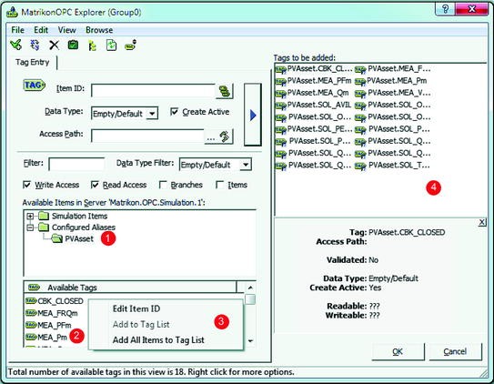

  

  MatrikonOPC server explorer—data tag configuration

• 7. Choose the “PVAsset” group from the “Available Items” tree view (marked ❶ in Fig. 16.12) and note that the tags imported into the OPC server are showing in the “Available Tags” list (marked ❷ in Fig. 16.12)

• 8. Right click in the “Available Tags” list view and choose “Add all items to tag list” from the context menu (marked ❸ in Fig. 16.12)

• 9. Note all the tags showing up in the “Tags to be added list” (marked ❹ in Fig. 16.12)

• 10. Click OK to add all the tags to the observation list in the OPC server explorer as shown in Fig. 16.13. Check that the qualities of tags are reading good and the values for the data tags are all zero. The values are zero because the simulation has not started; the OPC server has not received any values from the PowerFactory simulation engine.

  Fig. 16.13

  

  MatrikonOPC server explorer—list of tags for observation and control

16.5.7 Configuring Solar Irradiance and Temperature Profile

As mentioned in the introductory discussion, ElmFile objects are often used to feed in system variables that change with respect to time. In the demo, solar irradiance and the temperature are such variables. The package provided with this chapter has two files containing time series data for irradiance and temperature; the names of the files are “MeasuredSolarIrradianceProfile.txt” and “MockedUpTempratureProfile.txt.” The screenshot in Fig. 16.14 shows the list of ElmFile objects used in the sample project and one of its edits showing the parameter to choose the appropriate file.

Fig. 16.14

Screenshot showing required ElmFile objects and the parameter to configure the time-series.csv file

16.5.8 Initializing the System

This demonstration utilizes the RMS simulation feature in PowerFactory to simulate a real-world PV system. Initialization object and its configuration play an important role in the time domain simulation. The following section of the chapter briefly explains the initialization of the demonstration model and other interesting options available via the initialization object.

• 1. Ensure that the RMS/EMT simulation toolbox is selected in the toolbar. If it is not selected, use the “Change toolbox” drop-down button (marked ❶ in Fig. 16.15) and choose “RMS/EMT Simulation” (marked ❷ in Fig. 16.15).

  Fig. 16.15

  

  PowerFactory toolbar showing RMS simulation toolbox

• 2. Ensure that the OPC link object in PowerFactory is linked to the OPC server as explained in earlier sections of this chapter.

• 3. Click the “Events” button (marked ❺ in Fig. 16.15) to open the events list created in the previous simulation session and delete all of them (if any).

• 4. Click the “Initialization” button (marked ❸ in Fig. 16.15) to bring up the initialization command object editor as shown in Fig. 16.16. Readers are highly encouraged to spend some time investigating various important options or user configurable parameters offered by the initialization objects such as the following:⁹

  Fig. 16.16

  

  Initialization command editor

  • Simulation method (RMS or EMT)

  • Network representation (balanced or unbalanced)

  • Load flows options

  • Integration step size configuration (setting a bigger step size speeds up the simulation)

  • Simulation start time

  • Real-time synchronization

  • Iteration control parameters

  • OPC read/write intervals, etc.

  Manipulating these parameters opens up numerous possibilities for RMS/EMT simulation in PowerFactory. Technical reference [4] supplied by DIgSILENT explains all the options in detail.

• 5. Click “Execute” to calculate initial condition.

• 6. Note that the “Value” column in the OPC server explorer has started showing the values as communicated by the external measurement objects (see Fig. 16.17).

  Fig. 16.17

  

  Matrikon OPC server explorer—list of tags after initialization

16.5.9 Running the Simulation

• 1. Click “Start Simulation” button (marked ❹ in Fig. 16.15 to bring up the simulation object editor.

• 2. Enter the number of seconds for which you need to simulate the system in the text box next to the “Absolute” label in the command editor.

• 3. Click “Execute” to run the simulation.

• 4. Switch to “Virtual Instrument Panel” in the graphic board to observe the P and Q production plot against time in the x-axis as shown in Fig. 16.21.

• 5. At the same time, note that the values of the OPC are rapidly changing in real time as the simulation is running (refer Fig. 16.17 )

16.6 Controlling the Model Using OPC Server Explorer

Following procedure explains how to control the model using the OPC server explorer (substituting for a real-world power system controller). For the demonstration, the following control actions should be executed from the MatrikonOPC server explorer.

• 1. Make sure the simulation is running.

• 2. Look at the OPC server and ensure that the value for “PVAsset-SOL_OFFCmd” is reading zero. Right click on the tag point and select “Write Values” from the context menu.

• 3. In the pop-up window, enter 1 (signal—high) for the “New Value” and click OK. Note the messages in PowerFactory output window, which reads as Fig. 16.18.

  Fig. 16.18

  

  PowerFactory output showing switching-off sequence

• 4. Also check that both P and Q output go to zero (see marker ❶ in Fig. 16.21).

• 5. Make sure to reset the value of “PVAsset_SOL_OFFCmd” to zero. If you do not, the switch-on control will not close the breakers.

• 6. To switch the PV system back into the grid, change the value of “PVAsset_SOL_ONCmd” to 1 (high).

• 7. Observe the following messages in the output window (see Fig. 16.19) and change in P and Q output of the PV generator (see marker ❷ in Fig. 16.21).

  Fig. 16.19

  

  PowerFactory output showing switching-on sequence

• 8. Readers can exercise the Q dispatch control by following the steps explained below:

  • To change the Q dispatch mode, set the value of “PVAsset_SOL_QMDCmd” to 2 using the OPC server explorer as explained. The model understands the number 2 as a command for base-load mode.

  • Next, change the set point (PVAsset_SOL_QSPCmd) to, say, 200 kVAr. The model is capable of converting the number 200 to its P.U. value.

  • Check the output window for messages about the change in Q mode and Q set point (see Fig. 16.20).

    Fig. 16.20

    

    PowerFactory output showing change in Q mode and set point

  • P and Q dispatch in the virtual instrument panel also reflects the change in Q mode and Q set point as shown under marker ❸ in Fig. 16.21.

    Fig. 16.21

    

    Plots showing P and Q produced by the PV plant in the demonstration system

16.7 Conclusion

Equipped with great features and wide range of calculation and event simulating capabilities, DIgSILENT’s PowerFactory comes in as a handy substitute to costly hardware in prototype developments and HIL testing. It also stands as a good substitute to super costly real-time digital simulators in simulating relatively smaller power systems. However, users need to take into account the following factors before using PowerFactory for prototyping and HIL testing.

• Modeling system dynamics—accuracy of simulation results compared to its measured values greatly depends on the precision with which the dynamics of the system is represented. However, the more the details in the model, simulations take longer time to solve. Thus, users have to make conscious effort on what is important in terms of system modeling for a given problem.

• The size of the network—size of the network also dictates the simulation speed. In many cases, it is possible to reduce large portions of the given power system and represents them by its simplified equivalents. However users have to be aware of the fact that; replacing a portion of the network with its equivalent can have significant effect on the simulation results.

• Integration step size or time step—step size must be chosen such that the simulation accurately represents the system frequency response up to the fastest transient of interest. Thus, the step size has to be worked out on a case-by-case basis.

• Synchronization between simulation time step and real time step. However, both in the case of controller prototyping and HIL testing, the setup is an off-line setup and thus time synchronization is not an issue.

• PowerFactory’s inability to connect to more than one OPC server—a shortcoming which can be overcome by employing third-party OPC tunnelers.

In short, besides many other usages—PowerFactory can go a long way in model-based control system development, prototyping, and testing of power system controllers.

References

Bélanger J, Venne P, Paquin J-N (2010) White paper—the what, where and why of real-time simulation. Opal-RT Technologies, Montréal, Oct 2010. Available from http://www.opal-rt.com/sites/default/files/technical_papers/PES-GM-Tutorial_04%20-%20Real%20Time%20Simulation.pdf. Accessed 08 Dec 2014
Theologitis IT (2011) Comparison of existing PV models and possible integration under EU grid specifications, Master of Science thesis, KTH School of Electrical Engineering, Division of Electrical Power Systems EPS-2011, SE-100 44 Stockholm, Jun 2011, XR-EE-ES 2011:011
Mahmood F Improving Photo-voltaic Model in PowerFactory, Degree Project, KTH School of Electrical Engineering, Division of Electrical Power Systems EPS-2012, SE-100 44 Stockholm, Nov. 2012, XR-EE-ES 2012:017
DIgSILENT PowerFactory 15.0 user manual and technical references (Licensed users can download latest user manual and technical references from http://www.digsilent.de/index.php/downloads.html)
Author information
Authors and Affiliations
Corresponding author
Editor information
Editors and Affiliations
16.1 Electronic Supplementary Material
Below is the link to the electronic supplementary material.
Rights and permissions
Copyright information
© 2014 Springer International Publishing Switzerland
About this chapter
Cite this chapter
Srinivasan, R. (2014). PowerFactory as a Software Stand-in for Hardware in Hardware-In-Loop Testing. In: Gonzalez-Longatt, F., Luis Rueda, J. (eds) PowerFactory Applications for Power System Analysis. Power Systems. Springer, Cham. https://doi.org/10.1007/978-3-319-12958-7_16
Download citation
DOI: https://doi.org/10.1007/978-3-319-12958-7_16
Published:
Publisher Name: Springer, Cham
Print ISBN: 978-3-319-12957-0
Online ISBN: 978-3-319-12958-7
eBook Packages: EnergyEnergy (R0)