SIMLAB Software for Uncertainty and Sensitivity Analysis

Abstract

SIMLAB 4.0 is a comprehensive stand-alone software package for performing global sensitivity analysis. Several sampling strategies and sensitivity measures are available. SIMLAB includes the most recent variance-based formulas for first-order and total-order sensitivity indices, graphical methods, as well as more classical methods. The peculiarity of SIMLAB, in contrast to previous versions of the package, is the possibility to run sequential sensitivity analysis, which allows updating the sensitivity measures at each run, or group of runs, of the model. The techniques can be accessed through the R environment as well as through a graphical user interface. The user can also add new techniques by simply adding the corresponding R code to the core layer. SIMLAB can be downloaded for free from the Joint Research Centre’s website.

1 Introduction

SIMLAB 4.0 is a newly implemented version of a software framework for uncertainty and sensitivity analysis. SIMLAB is the property of the Joint Research Centre (JRC) of the European Commission, which has financed its design and development since its first version, made available back in 1999. With this product, the JRC aims to employ up-to-date tools and practices of global sensitivity analysis in order to disseminate the culture of sensitivity analysis to an ever-increasing number of customers. In agreement with the EC dissemination policy, SIMLAB is publicly available for use by any person, company, or organization that downloads, installs, and uses the software , according to an end user software license agreement.

SIMLAB is available on the website of the Econometrics and Applied Statistics research group of the European Commission’s Joint Research Centre [3].

SIMLAB contains a set of techniques to execute global sensitivity analysis (GSA), primarily by Monte Carlo and sampling-based methods (as opposed to emulator/metamodel-based methods). No local sensitivity analysis tools are present in the software. The conceptual framework of GSA and the techniques available to perform GSA are described in Sobol’ (variance-based) sensitivity indices: theory and estimation algorithms. In summary, GSA is based on performing multiple model evaluations with a probabilistically-selected model input and then using the results of these evaluations to quantify the relative importance of the inputs in determining the uncertainty of the model output.

The tool, running in a 64-bit environment under Windows, is delivered as a self-installing setup. It provides a set of transparent, well-commented, and self-maintainable functions, coded in the R environment, that implement GSA techniques. The user can work both in the R environment by calling the R functions and, on the pre-compiled functions, through a graphical user interface (GUI) , developed in C# for the.NET framework, which facilitates the use of the application and allows to visually present the results of the sensitivity analysis .

The R package acts as the core layer of the application and contains all the algorithms and methods of global sensitivity analysis , with source codes available to the user. SIMLAB can easily be extended with new GSA techniques by adding the corresponding R code to the core layer. Modifications and maintenance of the core algorithms can be carried out by the user.

The GUI is built on top of a control layer, developed in C++, which links the core layer in R with the GUI itself. The control layer is responsible for the correct management of the calls to R, given the instructions provided by the user through the GUI. The control layer also handles warning and error messages.

The system requires the installation of R. SIMLAB uses two R packages through which R and SIMLAB communicate: Rcpp and RInside. Other R packages are used for statistical operations: stats, pspearman, sensitivity, lhs, randtoolbox, and rngWELL. Those packages are automatically downloaded from the Comprehensive R Archive Network (https://cran.r-project.org/) during SIMLAB installation.

SIMLAB gathers a variety of routines, written by different authors in Matlab or R, that implement various GSA techniques. These routines are heterogeneously programmed and are harmonized and integrated in SIMLAB.

SIMLAB offers a test suite of three commonly used analytical functions that the user can employ to test the methods implemented in SIMLAB. These functions are described in this chapter.

With respect to previous versions, SIMLAB 4.0 offers a new functionality that allows the user to perform sequential sensitivity analysis . The sequential process is entirely managed by the control layer. Specifically, the user can run a number of iterations of the sequence composed by sample generation, model execution, and sensitivity estimation, thus obtaining continuous updates and convergence monitoring of the sensitivity analysis results in real time. In the sequential sensitivity analysis, the iteration is repeated until the user is satisfied with the results of the sensitivity analysis. The user does not need to specify ex ante how many sample points to use in the analysis. A visualization tool assists the user to monitoring the convergence of the sensitivity results. This approach has the advantage of stopping the analysis when the user is satisfied with the level of precision of the GSA results, avoiding useless, and often expensive, extra model executions.

2 Installation

Requirements to install SIMLAB:

• A PC running Windows

• An internet connection

• R already installed

SIMLAB is currently only available for Windows. SIMLAB is written in C++, but uses packages from R . Therefore in order to use SIMLAB, the user must have both SIMLAB and R installed. It is recommended to install R prior to installing SIMLAB. R can be downloaded from https://cran.r-project.org/bin/windows/base/. Throughout the installation process, an internet connection is required.

To install SIMLAB, first unzip the Simlab_v4.rar file. In the folder SIMLAB Installation Files, run the setup.exe file. At this point, you may be asked to install Visual C++ Runtime Libraries. Since SIMLAB is dependent on these components, you must choose “Install” to continue. The SIMLAB Setup Wizard will now open automatically. Follow the instructions of the Wizard, including choosing a suitable directory for the installation. You will also be asked to nominate a folder which will be used for automatically depositing files to exchange information with R. Next, the Wizard will download and install the required R packages onto your R installation. This can also be done manually if desired. The following R packages are required to run SIMLAB:

• stats

• pspearman

• sensitivity

• lhs

• randtoolbox

• e1071

• mc2d

• rngWELL

Additional to these packages, SIMLAB installs its own package “SimLab4R” on R.

After installing the packages, automatically or otherwise, SIMLAB is installed and ready to run on your computer.

3 Data Workflow

Figure  57.1 below shows how data are processed by SIMLAB. The files for data exchange are represented by green boxes and contain ASCII text with an easy to understand format. These files contain information on the input distributions and their correlation structure, the generated sample (sample file), and the results of the model execution (simulated output). The setup of the input variables (i.e., the choice of the probability density functions and their parameters and the correlation matrix for the statistical characterization of input uncertainty) and the computer code implementing the simulation model are provided by the user (the blue boxes). The red boxes are the tools offered by SIMLAB: the sample generation step, the uncertainty analysis, and the GSA technique to compute the sensitivity indices. This latter is usually intimately related to the type of sampling used. SIMLAB also offers graphical tools to visualize the results of the GSA.

Fig. 57.1

SIMLAB data workflow (Courtesy of Federico Ferretti, Joint Research Centre, European Commission)

The core layer in R contains different functions that can be considered as building blocks for the GSA. Those functions allow the user to select among different types of sampling methods, to impose a desired correlation between inputs, to generate random samples from a set of assigned distributions, to evaluate the GSA measures according to the method selected, and to choose the stopping criterion for the GSA evaluation process. For example, the R command used to generate a log-uniformly distributed sample of size N with lower bound a and upper bound b is:

sam <- random(N,1)

qloguniform(sam,a,b)

The GUI facilitates the interaction of the user with the core layer. The GUI allows the user to save the working configuration for subsequent analyses to avoid the need to rerun the entire process. In particular, four working configurations can be saved: the definition of the model inputs (their number, their names, their probability distributions, and their correlation), the generated sample of inputs (with information on the type of sampling strategy used), the generated model output, and the evaluated sensitivity indices. A specific GUI functionality is dedicated to monitor the convergence of the sensitivity indices through a visualization tool.

The next version of SIMLAB will foresee the possibility to pause the sequential analysis and then restart it at a later stage.

4 Overview of Using SIMLAB

The first step of a GSA is to select ranges and probability density functions for the model inputs that are the object of the analysis. This is accomplished by the “Factors definition” function of the GUI. Here all the properties of the inputs are specified. It is possible to add new inputs, modifying or removing existing ones. The configuration of the model input can be saved to file and an existing configuration can be loaded into SIMLAB. Once the inputs have been defined it is also possible to specify a correlation matrix. See the next section for a summary of the probability density functions handled by SIMLAB.

The second step of the GSA is the sample generation. Four different sampling methods can be set: simple random, quasi-random, Latin hypercube, and the Sobol’ design. This latter is required if one is interested to compute Sobol’ sensitivity indices. As the GSA is executed sequentially in blocks of samples, the user is required to insert three values: the size of the first subsample, the size of the subsequent subsamples, and the maximum allowed sample size which, when reached, would terminate the GSA if not previously terminated. The generated sample can be saved to a file in ASCII format or as a csv file. The entire configuration composed by information on the input and generated sample can also be saved. The generated sample can be visualized as multiple histograms (one per input), cumulative histograms, 2D scatterplots (between pairs of inputs), and cobwebs (all inputs together).

In the third step “Output variables selection,” model output variable names are assigned. Multiple output variables and time-dependent variables can be handled.

Further, the user has to define a threshold value for the convergence criterion. The convergence criterion is based on the calculation of the absolute difference between each sensitivity index at step n − 1 and step n and on the calculation of the maximum of these absolute differences across all inputs and all outputs. The process will stop when this maximum difference gets smaller than the threshold value chosen by the user. Other convergence criteria will be added in the next release of SIMLAB.

The “model execution” step allows the user to link a model to SIMLAB. The user has to specify the name of an executable (the code of the model) that returns the model output variables with the names specified in the “output variables selection step.” SIMLAB foresees the possibility for the user to add a set of arguments needed by the model when launching the executable. The user has also to specify the name of the sample file from where the sample generated at the ith iteration will be read and the name of the output file where the results of the model output at the ith iteration will be saved. This latter specification is important in order not to lose the results of the model runs, which might be computationally intensive. The executable (the code of the model) has to foresee the reading from (writing to) the sample (output) file specified by SIMLAB. As such, SIMLAB will be able to run sequentially, generating a first subset of samples, running the model on this subset, and producing a subset of model outputs, which are saved to the output file and are used to obtain estimates of sensitivity indices of various nature.

The final two steps are “sensitivity evaluation” and “uncertainty evaluation,” the first being much more developed in SIMLAB. See the next section for an overview of the sensitivity analysis methods and the options offered by the uncertainty evaluation.

5 Available Techniques

Referring back to Fig. 57.1, the workflow of a sensitivity analysis consists of a number of steps. Fundamentally, SIMLAB performs two basic tasks of this workflow: generating the sample design that is used to specify the input values to each model run and post-processing the results of the model runs specified by the sample. For both of these operations, SIMLAB has a number of features which are outlined in this section.

5.1 Sampling

The selection of the sample design for a sensitivity analysis must be given some prior consideration, because the type of design dictates which measures of sensitivity can be estimated. The sensitivity measures that are associated with each design are described in the following section. The sample designs available in SIMLAB are as follows:

Simple random : :

this is simply a sequence of (pseudo-)random points taken from the input space–see Fig. 57.2. Random sampling has the advantage that sample replications can be taken, in order to estimate the error due to the sample size; however, random sampling is characterized by clustering of points which can reduce the efficiency of the design in terms of convergence in Monte Carlo applications.

Fig. 57.2

Simple random sampling in two dimensions with 128 points

Latin hypercube : :

this is the well-known sampling design proposed by [4], which has the property that sample points are quite evenly distributed with respect to each dimension – see Fig. 57.3. For a sample of n points, the range of each variable is divided into n equally spaced intervals. A sample point is taken by randomly selecting an interval from each dimension and then taking a random sample point from within the resulting hypercube. Intervals are sampled without replacement to ensure even distribution of points with respect to each variable. A drawback of Latin hypercube sampling is that an existing design cannot be extended to higher sample sizes without repositioning all sample points.

Fig. 57.3

Latin hypercube sampling in two dimensions with 128 points

Quasi-random : :

a so-called low-discrepancy sequence which has many of the properties of random numbers but ensures that points are well spaced in order to improve the rate of convergence of sensitivity estimates – see Fig. 57.4. Typically, quasi-random numbers will result in more accurate estimates of sensitivity at a given sample size. SIMLAB uses the Sobol’ (LP-τ) sequence [9], which also has the advantage that points can be added sequentially without restructuring the whole design. Note that the LP-τ sequence has particularly low discrepancy at sample values that are positive integer powers of 2, i.e., n = 2ⁱ, i = 1, 2, ….

Fig. 57.4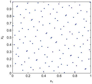

Sobol’ LP-τ sampling in two dimensions with 128 points

Sobol’ design : :

this is a structured design based on quasi-random sampling, structured in such a way as to allow estimation of variance-based sensitivity indices (first order and total order), via Monte Carlo integration – see Chapter 5 – and [10]. It is sometimes called “radial” sampling, since the design consists of a number n _r of smaller designs that each have k + 1 points (where k is the number of inputs of the model/function) that “radiate” from a single starting point – see Fig. 57.5. In fact, each of these smaller designs is equivalent to a set of k one-at-a-time designs, where each variable is perturbed individually. The total sample size (number of model runs) is therefore n = n _r (k + 1).

Fig. 57.5

Sobol’ radial design in three dimensions

FAST and Extended FAST design : :

these designs are also structured in such a way as to allow estimation of variance-based sensitivity indices: first-order indices for FAST [2], and both first-order and total-order indices for extended FAST [7]. FAST and extended FAST methods are not implemented sequentially in SIMLAB.

The sampling in all of the above designs can be performed with respect to the following distributions: discrete, uniform, piecewise uniform, log uniform, piecewise log uniform, normal, log normal, triangular, exponential, beta, gamma, and Weibull.

Before generating samples, the first step is to define the probability distributions of the input factors of the model. SIMLAB’s navigation pane is organized in steps which follow the logical workflow of a sensitivity analysis . Correspondingly, the first step is to go to the “ Factors definition” pane (Fig. 57.6). This gives an overview of each input factor. To start defining the distributions of input factors, click “Add new factor” and click “Edit” on the new factor that appears in the table. This opens a window as shown in Fig. 57.7. From here, the distribution type and parameters can be set, with information on the distribution given at the bottom of the window. Click “Save params” to save the distribution parameters to SIMLAB’s database. This process can be repeated for each input factor. Notice that every time a new factor is added, it appears as a subheading in the Factors definition heading of the navigation pane, allowing it to be edited at any time. A summary of all factors can be found by returning to the “Factors definition” window – see Fig. 57.8. Here the configuration of all factors can also be saved for use in other sessions or projects and similarly loaded from earlier work.

Fig. 57.6

The “Factors definition” pane

Fig. 57.7

Input distribution editing pane

Fig. 57.8

Input parameter summary pane

To actually generate a sample, go to the “Method” subheading of the “ Generation method definition” heading in the navigation pane. Here, the options for the sample generation can be set (see Fig. 57.9). The user must choose the method of sample generation using the “Method” and “Aux function” drop-down menus. Below, parameters can be set which control the sample size and optionally the step size in the sample generation, if a sequential sampling strategy is to be used. To perform an ordinary batch-mode sensitivity analysis (as opposed to sequential), set the “first subset size” option to the same number as the “maximum sample set size,” i.e., the total number of sample points. The “next subsets size” option should be set to zero. In the case of sequential sensitivity analysis, these settings can be used to control the step sizes for each iteration of sensitivity analysis.

Fig. 57.9

Sample method settings

Returning to the “Generation method definition” page, a summary of the variables and the sampling method is now displayed – see Fig. 57.10. To generate the sample, click “Generate and save whole sample.” At this point, the sample can be viewed in a number of ways by clicking the “View generated sample” button. A window will appear which allows the selection of factor, which can be selected by moving them to the “selected factors list” using the buttons – see Fig. 57.11. Histograms, cobwebs, and scatterplots can be generated depending on the number of variables selected. For example, with two factors selected, a scatterplot can be generated (Fig. 57.12), and with two or more variables, a cobweb plot can be created (Fig. 57.13). For the latter, values can be normalized or not by checking the box in the bottom right corner.

Fig. 57.10

Summary of sample and sample generation

Fig. 57.11

Displaying sample plots

Fig. 57.12

Scatterplot of one input variable against another

Fig. 57.13

Cobweb plot of three input variables without normalization

5.2 Model Execution

The “Model Execution” pane is presented in Fig. 57.14. SIMLAB is offered with three simple test models that can be found in the installation files. They allow the user to play and learn how to use the package. The first test model is the linear function of the form:

$$\displaystyle{Y =\sum _{ j=1}^{d}a_{ j}X_{j}}$$

Fig. 57.14

The aspect of the “Model Execution” pane

The a _j coefficients are selected by the user to decide upon the relative importance of the inputs. The marginal distributions of the X _j and their correlation matrix are selected by the user.

The second test model is the so-called Sobol’ g-function, a classical test function for which an analytical expression of the Sobol’ indices is available. Y = f ₁(X ₁) ×⋯ × f _k (X _k ) with $(X_{1},\ldots,X_{k}) \sim \mathcal{U}\, \left ([0,1]^{k}\right )$ and

$$\displaystyle{f_{j}(X_{j}) = \frac{\vert 4X_{j} - 2\vert + a_{j}} {1 + a_{j}},\ a_{j} \geq 0,\;j = 1,\ldots k.}$$

The a _j coefficients can be set by the user to decide upon the relative importance of the inputs. a _j = 0 corresponds to a very important input. As a _j increases, the relative importance of the input decreases.

The third test model is the so-called Ishigami function for which analytical Sobol’ indices are also available. The Ishigami function has the form: Y = sin(X ₁) + 7sin²(X ₂) + 0. 1X ⁴₃ sin(X ₁) with the three inputs uniformly distributed in the range (−π, π).

In the “Model Execution” pane, the test model is selected by clicking on “Browse” and choosing the executable file that implements the model. The executable file must also contain the instructions to read from the sample file and to write to the output file. For example, the executable file “LinearModel.exe” requires some arguments to be supplied by the user. These are the name of the input file, the name of the output file, and the coefficients a _i . If the user wants to run the sensitivity analysis of the linear model with coefficients a ₁ = 2, a ₂ = 7, a ₃ = 5, he has to prepare the “Model Execution” pane as depicted in Fig. 57.15.

Fig. 57.15

How to set up the “Model Execution” pane for the linear model

During the execution of a sequential sensitivity analysis, the sensitivity estimates obtained at a given iteration are compared with those obtained at the previous iteration. The convergence criterion is applied and, if convergence is not reached yet, the analysis proceeds. During this phase, the “Model Execution” pane looks as in Fig. 57.16.

Fig. 57.16

Sensitivity analysis in progress

5.3 Post-processing

The model must be run a number of times using one of the designs described in the previous section: this will return a vector of model output values. A number of measures of sensitivity can be estimated by SIMLAB based on the resulting model output values. Which measures can be estimated is dependent on the type of sampling design – see Fig. 57.17 for a summary.

Fig. 57.17

Compatibility of sampling methods with sensitivity measures

The methods supported by SIMLAB that are compatible with simple random, Latin hypercube, and quasi-random sampling are as follows (detailed descriptions of the methods are left to the references provided):

Standardized (rank) regression coefficients::

this involves fitting a simple linear regression to the sample data and then using the coefficients, standardized by their respective variances, as measures of sensitivity (Saltelli et al. 2000). This approach is appealingly simple and can work with a large number of input variables. However, when the output of the model is nonlinear with respect to its inputs, sensitivity may be misrepresented.

Kolmogorov-Smirnov test::

sensitivity is measured by a statistical test which, after ordering with respect to a given variable and dividing the sample into two subsets, compares the distributions of each subset to see whether there is a significant difference. The degree of difference is taken as a measure of sensitivity [8].

Contribution to the sample mean plot::

a plot which shows how each input variable contributes to the sample mean by estimating the mean as the sample points are successively added, in order of the value of each input variable. The plots can be used as measures of sensitivity and give further information about the effects of specific quantiles of the input distributions [1].

Contribution to the sample variance plot::

these plots are the same concept as the contribution to the sample mean plots, but applied to the sample variance instead of the mean [11].

CUSUNORO::

a similar approach to the contribution to the sample mean, which proceeds by standardizing the ordered data to have zero mean and unit variance [6].

EASI: :

an algorithm that estimates first-order sensitivity indices using the fast Fourier transform [5].

The Sobol’ design is more specialized than the random or quasi-random sampling and is specifically intended for use in estimating variance-based sensitivity indices, in particular first-order and total-order sensitivity indices (see Chapter 5). Note that the output from the model can be in the form of a time series or a multidimensional variable (vector of outputs). SIMLAB can provide sensitivity indices for each time point or for each element of the vector of outputs.

In order to estimate the sensitivity measures discussed in this section, model output values must be available, corresponding to the value of the model output at each of the input points in the sample matrix. If the model is available as an executable file or perhaps reachable via the command line (e.g., via Matlab), SIMLAB can run the model automatically at each of the sample points and perform a sequential sensitivity analysis by gradually increasing the sample size until convergence has been reached. Alternatively, SIMLAB can read model output values in an ASCII format – this might be easier if the model is already set up to quickly read a matrix of input values. In this case, the file containing the model output values should be selected in the “Model execution” pane. Be sure that the file path is also specified. By clicking “Start Monte Carlo run,” SIMLAB uses the input and output samples to estimate all sensitivity measures.

To view the sensitivity measures, go to the “Sensitivity evaluation” heading in the navigation pane. The type of sensitivity measure can be selected from the drop-down menu at the top. The measures can be displayed either on a chart or in a table, although if the output is not time dependent, a table is usually more appropriate. Scatterplots can also be generated by clicking the “Visualise SA” button, for example, Fig. 57.18 shows a scatterplot of the output against one input variable.

Fig. 57.18

An example of a scatterplot of the model output against one of its inputs

The “Uncertainty evaluation” heading also gives information about the uncertainty in the model output, displaying a histogram, as well as giving measures of mean, variance, measures of skewness, and so on (see Fig. 57.19). Finally, by going to the “Visual SA” window, a range of visual indications of sensitivity can be plotted. Figure 57.20 shows a CUSUNORO plot for the three model inputs of the linear model shown previously. Other options that are available with a random or quasi-random sample are “contribution to sample mean” plots and “contribution to sample variance” plots.

Fig. 57.19

Histogram and statistics of output distribution

Fig. 57.20

Contribution to sample variance plot

6 Extending SIMLAB with R

SIMLAB may also be extended to use other functions and packages within R. This includes adding other types of distributions of input variables, as well as adding different convergence criteria, other sensitivity methods, and uncertainty indicators.

In order to make such extensions, it is necessary to edit the R project source file “SimLab4R,” which forms the technical basis of the SIMLAB installation. This must be done via RStudio. This file will be available either as part of the SIMLAB installation or separately via the website.

The process of adding extensions is best illustrated by an example. Imagine that a new type of input distribution is required – the Cauchy distribution. The package that must be edited here is “simLabDistributions.R.” In this case, the following steps must be followed:

• 1. Add the name “Cauchy” in the list of distribution names in the getDistributions function.

• 2. Add the probability density function via the “dcauchy” function in the stats package. This is done by adding a call to “dcauchy” in the “getDensityFunction” function.

• 3. Add the inverse cumulative density function in the same way, by adding a line to call the “qcauchy” function from the “getInverseCDF” function.

• 4. Signal discrete and/or piecewise distribution if required, by adding lines to “isDensityPiecewise” and “isDensityDiscrete” (in this example not).

• 5. Define required parameters by adding a line to “getParameters.”

All the steps here are explained in more detail in the manual. Further possible steps include specifying default values and validity for parameters and specifying whether distributions allow truncation.

7 Conclusions

SIMLAB is a comprehensive stand-alone program for performing global sensitivity analysis, with a number of diverse sampling strategies and sensitivity measures available for estimation, both from classical methods and more recent research. It has the capacity for sequential analysis, and its GSA techniques can be accessed through the R environment, as well as through the graphical user interface. The user can add new GSA techniques by simply adding the corresponding R code to the core layer. SIMLAB can be downloaded for free from [3].

References

Bolado-Lavin, R., Castaings, W., Tarantola, S.: Contribution to the sample mean plot for graphical and numerical sensitivity analysis. Reliab. Eng. Syst. Saf. 94(6), 1041–1049 (2009)
Cukier, R., Levine, H., Shuler, K.: Nonlinear sensitivity analysis of multiparameter model systems. J. Comput. Phys. 26(1), 1–42 (1978)
European Commission SIMLAB: Sensitivity analysis software – Joint Research Centre. https://ec.europa.eu/jrc/en/samo/simlab (2015)
McKay, M., Beckman, R., Conover, W.: A comparison of three methods for selecting values of input variables in the analysis of output from a computer code. Technometrics 21, 239–245 (1979)
Plischke, E.: An effective algorithm for computing global sensitivity indices (EASI). Reliab. Eng. Syst. Saf. 95, 354–360 (2010)
Plischke, E.: An adaptive correlation ratio method using the cumulative sum of the reordered output. Reliab. Eng. Syst. Saf. 107, 149–156 (2012)
Saltelli, A., Tarantola, S., Chan, K.: Quantitative model-independent method for global sensitivity analysis of model output. Technometrics 41(1), 39–56 (1999)
Saltelli, A., Tarantola, S., Campolongo, F., Ratto, M.: Sensitivity Analysis in Practice. A Guide to Assessing Scientific Models. John Wiley and Sons, Chichester (2004)
Sobol’, I.M.: On the distribution of points in a cube and the approximate evaluation of integrals. USSR Comput. Math. Math. Phys. 7(4), 86–112 (1967)
Sobol’, I.M.: Sensitivity estimates for nonlinear mathematical models. Math. Model. Computat. Exp. 1(4), 407–414 (1993)
Tarantola, S., Kopustinskas, V., Bolado-Lavin, R., Kaliatka, A., Ušpuras, E., Vaišnoras, M.: Sensitivity analysis using contribution to sample variance plot: application to a water hammer model. Reliab. Eng. Syst. Saf. 99, 62–73 (2012)
Author information
Authors and Affiliations
Corresponding author
Editor information
Editors and Affiliations
Rights and permissions
Copyright information
© 2017 Springer International Publishing Switzerland
About this entry
Cite this entry
Tarantola, S., Becker, W. (2017). SIMLAB Software for Uncertainty and Sensitivity Analysis. In: Ghanem, R., Higdon, D., Owhadi, H. (eds) Handbook of Uncertainty Quantification. Springer, Cham. https://doi.org/10.1007/978-3-319-12385-1_61
Download citation
DOI: https://doi.org/10.1007/978-3-319-12385-1_61
Published:
Publisher Name: Springer, Cham
Print ISBN: 978-3-319-12384-4
Online ISBN: 978-3-319-12385-1
eBook Packages: Mathematics and StatisticsReference Module Computer Science and Engineering