
Abstract
Most signals we deal with in practice are random (unpredictable or erratic) and not deterministic. Random signals are encountered in one form or another in every practical communication system. They occur in communication both as information-conveying signal and as unwanted noise signal.
Philosophy is a game with objectives and no rules. Mathematics is a game with rules and no objectives.
—Anonymous
Access provided by Autonomous University of Puebla. Download chapter PDF
Keywords
- Probability Density Function
- Probability Density Function
- Cumulative Distribution Function
- Central Limit Theorem
- Joint Probability Density Function
These keywords were added by machine and not by the authors. This process is experimental and the keywords may be updated as the learning algorithm improves.
Most signals we deal with in practice are random (unpredictable or erratic) and not deterministic. Random signals are encountered in one form or another in every practical communication system. They occur in communication both as information-conveying signal and as unwanted noise signal.
A random quantity is one having values which are regulated in some probabilistic way.
Thus, our work with random quantities must begin with the theory of probability, which is the mathematical discipline that deals with the statistical characterization of random signals and random processes. Although the reader is expected to have had at least one course on probability theory and random variables, this chapter provides a cursory review of the basic concepts needed throughout this book. The concepts include probabilities, random variables, statistical averages or mean values, and probability models. A reader already versed in these concepts may skip this chapter.
2.1 Probability Fundamentals
A fundamental concept in the probability theory is the idea of an experiment. An experiment (or trial) is the performance of an operation that leads to results called outcomes. In other words, an outcome is a result of performing the experiment once. An event is one or more outcomes of an experiment. The relationship between outcomes and events is shown in the Venn diagram of Fig. 2.1.

Sample space illustrating the relationship between outcomes (points) and events (circles)
Thus,
An experiment consists of making a measurement or observation.
An outcome is a possible result of the experiment.
An event is a collection of outcomes.
An experiment is said to be random if its outcome cannot be predicted. Thus a random experiment is one that can be repeated a number of times but yields unpredictable outcome at each trial. Examples of random experiments are tossing a coin, rolling a die, observing the number of cars arriving at a toll booth, and keeping track of the number of telephone calls at your home. If we consider the experiment of rolling a die and regard event A as the appearance of the number 4. That event may or may not occur for every experiment.
2.1.1 Simple Probability
We now define the probability of an event. The probability of event A is the number of ways event A can occur divided by the total number of possible outcomes. Suppose we perform n trials of an experiment and we observe that outcomes satisfying event A occur nA times. We define the probability P(A) of event A occurring as
This is known as the relative frequency of event A. Two key points should be noted from Eq. (2.1). First, we note that the probability P of an event is always a positive number and that
where P = 0 when an event is not possible (never occurs) and P = 1 when the event is sure (always occurs). Second, observe that for the probability to have meaning, the number of trials n must be large.
If events A and B are disjoint or mutually exclusive, it follows that the two events cannot occur simultaneously or that the two events have no outcomes in common, as shown in Fig. 2.2.

Mutually exclusive or disjoint events
In this case, the probability that either event A or B occurs is equal to the sum of their probabilities, i.e.
To prove this, suppose in an experiments with n trials, event A occurs nA times, while event B occurs nB times. Then event A or event B occurs nA + nB times and
This result can be extended to the case when all possible events in an experiment are A, B, C, …, Z. If the experiment is performed n times and event A occurs nA times, event B occurs nB times, etc. Since some event must occur at each trial,
Dividing by n and assuming n is very large, we obtain
which indicates that the probabilities of mutually exclusive events must add up to unity. A special case of this is when two events are complimentary, i.e. if event A occurs, B must not occur and vice versa. In this case,
or
For example, in tossing a coin, the event of a head appearing is complementary to that of tail appearing. Since the probability of either event is ½, their probabilities add up to 1.
2.1.2 Joint Probability
Next, we consider when events A and B are not mutually exclusive. Two events are non-mutually exclusive if they have one or more outcomes in common, as illustrated in Fig. 2.3.

Non-mutually exclusive events
The probability of the union event A or B (or A + B) is
where P(AB) is called the joint probability of events A and B, i.e. the probability of the intersection or joint event AB.
2.1.3 Conditional Probability
Sometimes we are confronted with a situation in which the outcome of one event depends on another event. The dependence of event B on event A is measured by the conditional probability P(B∣A) given by
where P(AB) is the joint probability of events A and B. The notation B∣A stands “B given A.” In case events A and B are mutually exclusive, the joint probability P(AB) = 0 so that the conditional probability P(B∣A) = 0. Similarly, the conditional probability of A given B is
From Eqs. (2.9) and (2.10), we obtain
Eliminating P(AB) gives
which is a form of Bayes’ theorem.
2.1.4 Statistical Independence
Lastly, suppose events A and B do not depend on each other. In this case, events A and B are said to be statistically independent. Since B has no influence of A or vice versa,
From Eqs. (2.11) and (2.13), we obtain
indicating that the joint probability of statistically independent events is the product of the individual event probabilities. This can be extended to three or more statistically independent events
Example 2.1
Three coins are tossed simultaneously. Find: (a) the probability of getting exactly two heads, (b) the probability of getting at least one tail.
Solution
If we denote HTH as a head on the first coin, a tail on the second coin, and a head on the third coin, the 23 = 8 possible outcomes of tossing three coins simultaneously are the following:
The problem can be solved in several ways
-
Method 1: (Intuitive approach)
-
(a)
Let event A correspond to having exactly two heads, then
$$ \mathrm{Event}\ \mathrm{A}=\left\{\mathrm{HHT},\mathrm{HTH},\mathrm{THH}\right\} $$Since we have eight outcomes in total and three of them are in event A, then
$$ \mathrm{P}\left(\mathrm{A}\right)=3/8=0.375 $$ -
(b)
Let B denote having at least one tail,
$$ \mathrm{Event}\ \mathrm{B}=\left\{\mathrm{HTH},\mathrm{HHT},\mathrm{HTT},\mathrm{THH},\mathrm{TTH},\mathrm{THT},\mathrm{TTT}\right\} $$Hence,
$$ \mathrm{P}\left(\mathrm{B}\right)=7/8=0.875 $$
-
(a)
-
Method 2: (Analytic approach) Since the outcome of each separate coin is statistically independent, with head and tail equally likely,
$$ \mathrm{P}\left(\mathrm{H}\right)=\mathrm{P}\left(\mathrm{T}\right)={\textstyle \raisebox{1ex}{$1$}\!\left/ \!\raisebox{-1ex}{$2$}\right.} $$-
(a)
Event consists of mutually exclusive outcomes. Hence,
$$ \mathrm{P}\left(\mathrm{A}\right)=\mathrm{P}\left(\mathrm{HHT},\mathrm{HTH},\mathrm{THH}\right)=\left(\frac{1}{2}\right)\left(\frac{1}{2}\right)\left(\frac{1}{2}\right)+\left(\frac{1}{2}\right)\left(\frac{1}{2}\right)\left(\frac{1}{2}\right)+\left(\frac{1}{2}\right)\left(\frac{1}{2}\right)\left(\frac{1}{2}\right)=\frac{3}{8}=0.375 $$ -
(b)
Similarly,
$$ \mathrm{P}\left(\mathrm{B}\right)=\left(\mathrm{HTH},\mathrm{HHT},\mathrm{HTT},\mathrm{THH},\mathrm{TTH},\mathrm{THT},\mathrm{TTT}\right)=\left(\frac{1}{2}\right)\left(\frac{1}{2}\right)\left(\frac{1}{2}\right)+\mathrm{in}\ \mathrm{seven}\ \mathrm{places}=\frac{7}{8}=0.875 $$
-
(a)
Example 2.2
In a lab, there are 100 capacitors of three values and three voltage ratings as shown in Table 2.1. Let event A be drawing 12 pF capacitor and event B be drawing a 50 V capacitor. Determine: (a) P(A) and P(B), (b) P(AB), (c) P(A∣B), (d) P(B∣A).
Solution
-
(a)
From Table 2.1,
$$ \mathrm{P}\left(\mathrm{A}\right)=\mathrm{P}\left(12\ \mathrm{pF}\right)=36/100=0.36 $$and
$$ \mathrm{P}\left(\mathrm{B}\right)=\mathrm{P}\left(50\ \mathrm{V}\right)=41/100=0.41 $$ -
(b)
From the table,
$$ \mathrm{P}\left(\mathrm{AB}\right)=\mathrm{P}\left(12\ \mathrm{pF},50\ \mathrm{V}\right)=16/100=0.16 $$ -
(c)
From the table
$$ \mathrm{P}\left(\mathrm{A}\left|\mathrm{B}\right.\right)=\mathrm{P}\left(12\ \mathrm{pF}\left|50\ \mathrm{V}\right.\right)=16/41=0.3902 $$Check: From Eq. (2.10),
$$ P\left(A\Big|B\right)=\frac{P(AB)}{P(B)}=\frac{16/100}{41/100}=0.3902 $$ -
(d)
From the table,
$$ \mathrm{P}\left(\mathrm{B}\left|\mathrm{A}\right.\right)=\mathrm{P}\left(50\ \mathrm{V}\left|12\ \mathrm{pF}\right.\right)=16/36=0.4444 $$Check: From Eq. (2.9),
$$ P\left(B\Big|A\right)=\frac{P(AB)}{P(A)}=\frac{16/100}{36/100}=0.4444 $$
2.2 Random Variables
Random variables are used in probability theory for at least two reasons [1, 2]. First, the way we have defined probabilities earlier in terms of events is awkward. We cannot use that approach in describing sets of objects such as cars, apples, and houses. It is preferable to have numerical values for all outcomes. Second, mathematicians and communication engineers in particular deal with random processes that generate numerical outcomes. Such processes are handled using random variables.
The term “random variable” is a misnomer; a random variable is neither random nor a variable. Rather, it is a function or rule that produces numbers from the outcome of a random experiment. In other words, for every possible outcome of an experiment, a real number is assigned to the outcome. This outcome becomes the value of the random variable. We usually represent a random variable by an uppercase letters such as X, Y, and Z, while the value of a random variable (which is fixed) is represented by a lowercase letter such as x, y, and z. Thus, X is a function that maps elements of the sample space S to the real line − ∞ ≤ x ≤ ∞, as illustrated in Fig. 2.4.

Random variable X maps elements of the sample space to the real line
A random variable X is a single-valued real function that assigns a real value X(x) to every point x in the sample space.
Random variable X may be either discrete or continuous. X is said to be discrete random variable if it can take only discrete values. It is said to be continuous if it takes continuous values. An example of a discrete random variable is the outcome of rolling a die. An example of continuous random variable is one that is Gaussian distributed, to be discussed later.
2.2.1 Cumulative Distribution Function
Whether X is discrete or continuous, we need a probabilistic description of it in order to work with it. All random variables (discrete and continuous) have a cumulative distribution function (CDF).
The cumulative distribution function (CDF) is a function given by the probability that the random variable X is less than or equal to x, for every value x.
Let us denote the probability of the event X ≤ x, where x is given, as P(X ≤ x). The cumulative distribution function (CDF) of X is given by
for a continuous random variable X. Note that FX(x) does not depend on the random variable X, but on the assigned value of X. FX(x) has the following five properties:
-
1.
$$ {\mathrm{F}}_{\mathrm{X}}\left(-\infty \right)=0 $$(2.17a)
-
2.
$$ {\mathrm{F}}_{\mathrm{X}}\left(\infty \right)=1 $$(2.17b)
-
3.
$$ 0\le {\mathrm{F}}_{\mathrm{X}}\left(\mathrm{x}\right)\le 1 $$(2.17c)
-
4.
$$ {\mathrm{F}}_{\mathrm{X}}\left({\mathrm{x}}_1\right)\le {\mathrm{F}}_{\mathrm{X}}\left({\mathrm{x}}_2\right),\kern1em \mathrm{if}\kern0.5em {\mathrm{x}}_1<{\mathrm{x}}_2 $$(2.17d)
-
5.
$$ {\mathrm{P}\Big(\mathrm{x}}_1<\mathrm{X}\le {\mathrm{x}}_2\Big)={\mathrm{F}}_{\mathrm{X}}\left({\mathrm{x}}_2\right)-{\mathrm{F}}_{\mathrm{X}}\left({\mathrm{x}}_1\right) $$(2.17e)
The first and second properties show that the FX(−∞) includes no possible events and FX(∞) includes all possible events. The third property follows from the fact that FX(x) is a probability. The fourth property indicates that FX(x) is a nondecreasing function. And the last property is easy to prove since
or
If X is discrete, then
where P(xi) = P(X = xi) is the probability of obtaining event xi, and N is the largest integer such that x N ≤ x and N ≤ M, and M is the total number of points in the discrete distribution. It is assumed that x 1 < x 2 < x 3 < ⋅ ⋅ ⋅ < x M .
2.2.2 Probability Density Function
It is sometimes convenient to use the derivative of FX(x), which is given by
or
where fX(x) is known as the probability density function (PDF). Note that fX(x) has the following properties:
-
1.
$$ {\mathrm{f}}_{\mathrm{X}}\left(\mathrm{x}\right)\ge 0 $$(2.21a)
-
2.
$$ {\displaystyle \underset{-\infty }{\overset{\infty }{\int }}{f}_X(x) dx=1} $$(2.21b)
-
3.
$$ P\left({x}_1\le x\le {x}_2\right)={\displaystyle \underset{x_1}{\overset{x_2}{\int }}{f}_X(x) dx} $$(2.21c)
Properties 1 and 2 follows from the fact that \( {\rm F_X} \)(−∞) = 0 and \( {\rm F_X} \)(∞) = 1 respectively. As mentioned earlier, since \( {\rm F_X} \)(x) must be nondecreasing, its derivative \( {\rm f_X} \)(x) must always be nonnegative, as stated by Property 1. Property 3 is easy to prove. From Eq. (2.18),
which is typically illustrated in Fig. 2.5 for a continuous random variable.

A typical PDF
For discrete X,
where M is the total number of discrete events, P(xi) = P(x = xi), and δ(x) is the impulse function. Thus,
The probability density function (PDF) of a continuous (or discrete) random variable is a function which can be integrated (or summed) to obtain the probability that the random variable takes a value in a given interval.
2.2.3 Joint Distribution
We have focused on cases when a single random variable is involved. Sometimes several random variables are required to describe the outcome of an experiment. Here we consider situations involving two random variables X and Y; this may be extended to any number of random variables. The joint cumulative distribution function (joint cdf) of X and Y is the function
where \( -\infty <x<\infty, -\infty <y<\infty \). If FXY(x,y) is continuous, the joint probability density function (joint PDF) of X and Y is given by
where fXY(x,y) ≥ 0. Just as we did for a single variable, the probability of event x 1 < X ≤ x 2 and y 1 < Y ≤ y 2 is
From this, we obtain the case where the entire sample space is included as
since the total probability must be unity.
Given the joint CDF of X and Y, we can obtain the individual CDFs of the random variables X and Y. For X,
and for Y,
FX(x) and FY(y) are known as the marginal cumulative distribution functions (marginal CDFs).
Similarly, the individual PDFs of the random variables X and Y can be obtained from their joint PDF. For X,
and for Y,
fX(x) and fY(y) are known as the marginal probability density functions (marginal PDFs).
As mentioned earlier, two random variables are independent if the values taken by one do not affect the other. As a result,
or
This condition is equivalent to
Thus, two random variables are independent when their joint distribution (or density) is the product of their individual marginal distributions (or densities).
Finally, we may extend the concept of conditional probabilities to the case of continuous random variables. The conditional probability density function (conditional PDF) of X given the event Y = y is
where fY(y) is the marginal PDF of Y. Note that fX(x∣Y = y) is a function of x with y fixed. Similarly, the conditional PFD of Y given X = x is
where fX(x) is the marginal PDF of X. By combining Eqs. (2.34) and (2.36), we get
which is Bayes’ theorem for continuous random variables. If X and Y are independent, combining Eqs. (2.34)–(2.36) gives
indicating that one random variable has no effect on the other.
Example 2.3
An analog-to-digital converter is an eight-level quantizer with the output of 0, 1, 2, 3, 4, 5, 6, 7. Each level has the probability given by
(a) Sketch FX(x) and fX(x). (b) Find P(X ≤ 1), P(X > 3), (c) Determine P(2 ≤ X ≤ 5).
Solution
-
(a)
The random variable is discrete. Since the values of x are limited to 0 ≤ x ≤ 7,
$$ {\mathrm{F}}_{\mathrm{X}}\left(-1\right)=\mathrm{P}\left(\mathrm{X}<-1\right)=0 $$$$ {\mathrm{F}}_{\mathrm{X}}(0)=\mathrm{P}\left(\mathrm{X}\le 0\right)=1/8 $$$$ {\mathrm{F}}_{\mathrm{X}}(1)=\mathrm{P}\left(\mathrm{X}\le 1\right)=\mathrm{P}\left(\mathrm{X}=0\right)+\mathrm{P}\left(\mathrm{X}=1\right)=2/8 $$$$ {\mathrm{F}}_{\mathrm{X}}(2)=\mathrm{P}\left(\mathrm{X}\le 2\right)=\mathrm{P}\left(\mathrm{X}=0\right)+\mathrm{P}\left(\mathrm{X}=1\right)+\mathrm{P}\left(\mathrm{X}=2\right)=3/8 $$Thus, in general
$$ {F}_X(i)=\left\{\begin{array}{c}\hfill \left(i+1\right)/8,\begin{array}{cc}\hfill \hfill & \hfill 2\le i\le 7\hfill \end{array}\hfill \\ {}\hfill 1,\begin{array}{cc}\hfill \hfill & \hfill i>7\hfill \end{array}\hfill \end{array}\right. $$(2.3.1)The distribution function is sketched in Fig. 2.6a. Its derivative produces the PDF, which is given by
Fig. 2.6 
For Example 2.3: (a) distribution function of X, (b) probability density function of X
$$ {f}_X(x)={\displaystyle \sum_{i=0}^7\delta \left(x-i\right)/8} $$(2.3.2)and sketched in Fig. 2.6b.
-
(b)
We already found P(X ≤ 1) as
$$ \mathrm{P}\left(\mathrm{X}\le 1\right)=\mathrm{P}\left(\mathrm{X}=0\right)+\mathrm{P}\left(\mathrm{X}=1\right)=1/4 $$$$ \mathrm{P}\left(\mathrm{X}>3\right)=1-\mathrm{P}\left(\mathrm{X}\le 3\right)=1-{\mathrm{F}}_{\mathrm{X}}(3) $$But
$$ \kern7pt {\mathrm{F}}_{\mathrm{X}}(3)=\mathrm{P}\left(\mathrm{X}\le 3\right)=\mathrm{P}\left(\mathrm{X}=0\right)+\mathrm{P}\left(\mathrm{X}=1\right)+\mathrm{P}\left(\mathrm{X}=2\right)+\mathrm{P}\left(\mathrm{X}=3\right)=4/8 $$We can also obtain this from Eq. (2.3.1). Hence,
$$ \mathrm{P}\left(\mathrm{X}>3\right)=1-4/8={\scriptscriptstyle \frac{1}{2}}. $$ -
(c)
For P(2 ≤ X ≤ 5), using Eq. (2.3.1)
$$ \mathrm{P}\left(2\le \mathrm{X}\le 5\right)={\mathrm{F}}_{\mathrm{X}}(5)-{\mathrm{F}}_{\mathrm{X}}(2)=5/8-2/8=3/8. $$

Example 2.4
The CDF of a random variable is given by
(a) Sketch FX(x) and fX(x). (b) Find P(X ≤ 4) and P(2 < X ≤ 7).
Solution
-
(a)
In this case, X is a continuous random variable. FX(x) is sketched in Fig. 2.7a. We obtain the PDF of X by taking the derivative of FX(x), i.e.
Fig. 2.7 
For Example 2.4: (a) CDF, (b) PDF
$$ {f}_X(x)=\left\{\begin{array}{c}\hfill 0,\begin{array}{cc}\hfill \hfill & \hfill \hfill \end{array}x<1\hfill \\ {}\hfill \frac{1}{8},\begin{array}{cc}\hfill \hfill & \hfill 1\le x<9\hfill \end{array}\hfill \\ {}\hfill 0,\begin{array}{cc}\hfill \hfill & \hfill x\ge 9\hfill \end{array}\hfill \end{array}\right. $$which is sketched in Fig. 2.7b. Notice that fX(x) satisfies the requirement of a probability because the area under the curve in Fig. 2.7b is unity. A random number having a PDF such as shown in Fig. 2.7b is said to be uniformly distributed because fX(x) is constant within 1 and 9.
-
(b)
\( P\left(X\le 4\right)={F}_X(4)=3/8 \)
$$ P\left(2<x\le 7\right)={F}_X(7)-{F}_X(2)=6/8-1/8=5/8 $$

Example 2.5
Given that two random variables have the joint PDF
(a) Evaluate k such that the PDF is a valid one. (b) Determine FXY(x,y). (c) Are X and Y independent random variables? (d) Find the probabilities that X ≤ 1 and Y ≤ 2. (e) Find the probability that X ≤ 2 and Y > 1.
Solution
-
(a)
In order for the given PDF to be valid, Eq. (2.27) must be satisfied, i.e.
$$ {\displaystyle \underset{-\infty }{\overset{\infty }{\int }}{\displaystyle \underset{-\infty }{\overset{\infty }{\int }}{f}_{XY}\left(x,y\right) dxdy}}=1 $$so that
$$ 1={\displaystyle \underset{0}{\overset{\infty }{\int }}{\displaystyle \underset{0}{\overset{\infty }{\int }}k{e}^{-\left(x+2y\right)} dx dy}}=k{\displaystyle \underset{0}{\overset{\infty }{\int }}{e}^{-x} dx}{\displaystyle \underset{0}{\overset{\infty }{\int }}{e}^{-2y} dy}=k(1)\left(\frac{1}{2}\right)\begin{array}{cc}\hfill \hfill & \hfill \hfill \end{array} $$Hence, k = 2.
-
(b)
\( {F}_{XY}\left(x,y\right)={\displaystyle \underset{0}{\overset{x}{\int }}{\displaystyle \underset{0}{\overset{y}{\int }}2{e}^{-\left(x+2y\right)} dx dy}}=2{\displaystyle \underset{0}{\overset{x}{\int }}{e}^{-x} dx}{\displaystyle \underset{0}{\overset{y}{\int }}{e}^{-2y} dy}=\left({e}^{-x}-1\right)\left({e}^{-2y}-1\right)={F}_X(x){F}_Y(y)\begin{array}{cc}\hfill \hfill & \hfill \hfill \end{array} \)
-
(c)
Since the joint CDF factors into individual CDFs, we conclude that the random variables are independent.
-
(d)
\(P\left(X\le 1,Y\le 2\right)={\displaystyle \underset{x=0}{\overset{1}{\int }}{\displaystyle \underset{y=0}{\overset{2}{\int }}{f}_{XY}\left(x,y\right) dxdy}}=2{\displaystyle \underset{0}{\overset{1}{\int }}{e}^{-x} dx{\displaystyle \underset{0}{\overset{2}{\int }}{e}^{-2y} dy}=\left(1-{e}^{-1}\right)\left(1-{e}^{-4}\right)}=0.6205 \)
-
(e)
\( P\left(X\le 2,Y>1\right)={\displaystyle \underset{x=0}{\overset{2}{\int }}{\displaystyle \underset{y=1}{\overset{\infty }{\int }}{f}_{XY}\left(x,y\right) dxdy}}=2{\displaystyle \underset{0}{\overset{2}{\int }}{e}^{-x} dx{\displaystyle \underset{1}{\overset{\infty }{\int }}{e}^{-2y} dy}=\left({e}^{-2}-1\right)\left({e}^{-2}\right)}=0.117 \)
2.3 Operations on Random Variables
There are several operations that can be performed on random variables. These include the expected value, moments, variance, covariance, correlation, and transformation of the random variables. The operations are very important in our study of computer communications systems. We will consider some of them in this section, while others will be covered in later sections. We begin with the mean or average values of a random variable.
2.3.1 Expectations and Moments
Let X be a discrete random variable which takes on M values x 1, x 2, x .3, ⋯, x M that respectively occur n 1, n 2, n .3, ⋯, n M in n trials, where n is very large. The statistical average (mean or expectation) of X is given by
But by the relative-frequency definition of probability in Eq. (2.1), ni/n = P(xi). Hence, the mean or expected value of the discrete random variable X is
where E stands for the expectation operator.
If X is a continuous random variable, we apply a similar argument. Rather than doing that, we can replace the summation in Eq. (2.40) with integration and obtain
where fX(x) is the PDF of X.
In addition to the expected value of X, we are also interested in the expected value of functions of X. In general, the expected value of a function g(X) of the random variable X is given by
for continuous random variable X. If X is discrete, we replace the integration with summation and obtain
Consider the special case when g(x) = X n. Equation (2.42) becomes
E(Xn) is known as the nth moment of the random variable X. When n = 1, we have the first moment \( \overline{X} \) as in Eq. (2.42). When n = 2, we have the second moment \( \overline{X^2} \) and so on.
2.3.2 Variance
The moments defined in Eq. (2.44) may be regarded as moments about the origin, We may also define central moments, which are moments about the mean value m X = E(X) of X. If X is a continuous random variable,
It is evident that the central moment is zero when n = 1. When n = 2, the second central moment is known as the variance σ 2 X of X, i.e.
If X is discrete,
The square root of the variance (i.e. σ X ) is called the standard deviation of X. By expansion,
or
Note that from Eq. (2.48) that if the mean mX = 0, the variance is equal to the second moment E[X2].
2.3.3 Multivariate Expectations
We can extend what we have discussed so far for one random variable to two or more random variables. If g(X,Y) is a function of random variables X and Y, its expected value is
Consider a special case in which g(X,Y) = X + Y, where X and Y need not be independent, then
indicating the mean of the sum of two random variables is equal to the sum of their individual means. This may be extended to any number of random variables.
Next, consider the case in which g(X,Y) = XY, then
If X and Y are independent,
implying that the mean of the product of two independent random variables is equal to the product of their individual means.
2.3.4 Covariance and Correlation
If we let g(X,Y) = X n Y k, the generalized moments are defined as
We notice that Eq. (2.50) is a special case of Eq. (2.54). The joint moments in Eqs. (2.52) and (2.54) are about the origin. The generalized central moments are defined by
The sum of n and k is the order of the moment. Of particular importance is the second central moment (when n = k = 1) and it is called covariance of X and Y, i.e.
or
Their correlation coefficient ρ XY is given by
where − 1 ≤ ρ XY ≤ 1. Both covariance and correlation coefficient serve as measures of the interdependence of X and Y. ρ XY = 1 when Y = X and ρ XY = −1 when Y = −X. Two random variables X and Y are said to be uncorrelated if
and they are orthogonal if
If X and Y are independent, we can readily show that Cov(X,Y) = 0 = ρ XY . This indicates that when two random variables are independent, they are also uncorrelated.
Example 2.6
A complex communication system is checked on regular basis. The number of failures of the system in a month of operation has the probability distribution given in Table 2.2. (a) Find the average number and variance of failures in a month. (b) If X denotes the number of failures, determine mean and variance of Y = X + 1.
Solution
-
(a)
Using Eq. (2.40)
$$ \begin{array}{l}\overline{X}={m}_X={\displaystyle \sum_{i=1}^M{x}_iP}\left({x}_i\right)\\ {}\begin{array}{cc}\hfill \hfill & \hfill \hfill \end{array}\kern-5pt =0(0.2)+1(0.33)+2(0.25)+3(0.15)+4(0.05)+5(0.02)\\ {}\begin{array}{cc}\hfill \hfill & \hfill \hfill \end{array}\kern-5pt =1.58\end{array} $$To get the variance, we need the second moment.
$$ \begin{array}{l}\overline{X^2}=E\left({X}^2\right)={\displaystyle \sum_{i=1}^M{x}_i^2P}\left({x}_i\right)\\ {}\begin{array}{cc}\hfill \hfill & \hfill \hfill \end{array}={0}^2(0.2)+{1}^2(0.33)+{2}^2(0.25)+{3}^2(0.15)+{4}^2(0.05)+{5}^2(0.02)\\ {}\begin{array}{cc}\hfill \hfill & \hfill \hfill \end{array}=3.98\end{array} $$$$\mathrm{Var}(X)={\sigma}_X^2=E\left[{X}^2\right]-{m}_X^2=3.98-{1.58}^2=1.4836 $$ -
(b)
If Y = X + 1, then
$$ \begin{array}{l}\overline{Y}={m}_Y={\displaystyle \sum_{i=1}^M\left({x}_i+1\right)P}\left({x}_i\right)\\ {}\begin{array}{cc}\hfill \hfill & \hfill \hfill \end{array}\kern-5pt =1(0.2)+2(0.33)+3(0.25)+4(0.15)+5(0.05)+6(0.02)\\ {}\begin{array}{cc}\hfill \hfill & \hfill \hfill \end{array}\kern-5pt =2.58\end{array} $$Similarly,
$$ \begin{array}{l}\overline{Y^2}=E\left({Y}^2\right)={\displaystyle \sum_{i=1}^M{\left({x}_i+1\right)}^2P}\left({x}_i\right)\\ {}\begin{array}{cc}\hfill \hfill & \hfill \hfill \end{array}\kern-1pt ={1}^2(0.2)+{2}^2(0.33)+{3}^2(0.25)+{4}^2(0.15)+{5}^2(0.05)+{6}^2(0.02)\\ {}\begin{array}{cc}\hfill \hfill & \hfill \hfill \end{array}\kern-1pt =8.14\end{array} $$$$ \mathrm{Var}(Y)={\sigma}_y^2=E\left[{Y}^2\right]-{m}_Y^2=8.14-{2.58}^2=1.4836 $$which is the same as Var(X). This should be expected because adding a constant value of 1 to X does not change its randomness.
Example 2.7
Given a continuous random variable X with PDF
(a) Determine E(X) and E(X2). (b) Assuming that Y = 3X + 1, calculate E(Y) and Var(Y).
Solution
-
(a)
Using Eq. (2.41),
$$ \begin{array}{l}E(X)={\displaystyle \underset{-\infty }{\overset{\infty }{\int }}x{f}_X(x) dx}={\displaystyle \underset{0}{\overset{\infty }{\int }}x\left(2{e}^{-2x}\right) dx}\\ {}\begin{array}{cc}\hfill \hfill & \hfill \hfill \end{array}\kern7pt =2{\left[\frac{e^{-2x}}{4}\left(-2x-1\right)\right]}_0^{\infty }=\frac{1}{2}\end{array} $$$$ \begin{array}{l}E\left({X}^2\right)={\displaystyle \underset{-\infty }{\overset{\infty }{\int }}{x}^2{f}_X(x) dx}={\displaystyle \underset{0}{\overset{\infty }{\int }}{x}^2\left(2{e}^{-2x}\right) dx}\\ {}\begin{array}{cc}\hfill \hfill & \hfill \hfill \end{array}\kern12pt =2{\left[\frac{e^{-2x}}{-8}\left(4{x}^2+4x+2\right)\right]}_0^{\infty }=\frac{1}{2}\end{array} $$$$ \mathrm{Var}\left(\mathrm{X}\right)=E\left({X}^2\right)-{\left[E(X)\right]}^2=\frac{1}{2}-\frac{1}{4}=\frac{1}{4} $$ -
(b)
Rather than carrying out a similar complex integration, we can use common sense or intuitive argument to obtain E(Y) and E(Y2). Since Y is linearly dependent on X and the mean value of 1 is 1,
$$ \mathrm{E}\left(\mathrm{Y}\right)=\mathrm{E}\left(3\mathrm{X}+1\right)=3\mathrm{E}\left(\mathrm{X}\right)+\mathrm{E}(1)=3/2+1=5/2. $$Since the 1 in Y = 3X + 1 is constant, it does not affect the Var(Y). And because a square factor is involved in the calculation of variance,
$$ \mathrm{Var}\left(\mathrm{Y}\right)={3}^2\mathrm{Var}\left(\mathrm{X}\right)=9/4. $$We would have got the same thing if we have carried the integration in Eq. (2.45). To be sure this is the case,
$$ \begin{array}{l}E\left({Y}^2\right)={\displaystyle \underset{-\infty }{\overset{\infty }{\int }}{\left(3x+1\right)}^2{f}_X(x) dx}={\displaystyle \underset{-\infty }{\overset{\infty }{\int }}\left(9{x}^2+6x+1\right){f}_X(x) dx}\\ {}\begin{array}{cc}\hfill \hfill & \hfill \hfill \end{array}\kern12pt =9E\left({X}^2\right)+6E(X)+E(1)=\frac{9}{2}+\frac{6}{2}+1=\frac{17}{2}\end{array} $$$$ \mathrm{Var}(Y)=E\left({Y}^2\right)-{E}^2(Y)=\frac{17}{2}-\frac{25}{4}=\frac{9}{4} $$confirming our intuitive approach.
Example 2.8
X and Y are two random variables with joint PDF given by
(a) Find E(X + Y) and E(XY). (b) Compute Cov(X,Y) and ρ XY . (c) Determine whether X and Y are uncorrelated and/or orthogonal.
Solution
-
(a)
$$ \begin{array}{l}\overline{X+Y}=\kern.5pt E\left[X+Y\right]={\displaystyle \underset{-\infty }{\overset{\infty }{\int }}{\displaystyle \underset{-\infty }{\overset{\infty }{\int }}}\left(x+y\right){f}_{XY}(x) dx} dy={\displaystyle \underset{0}{\overset{1}{\int }}{\displaystyle \underset{0}{\overset{1}{\int }}}\left(x+y\right)\left(x+y\right) dx} dy\\ {}\begin{array}{cc}\hfill \hfill & \hfill \kern18pt =\hfill \end{array}{\displaystyle \underset{0}{\overset{1}{\int }}{\displaystyle \underset{0}{\overset{1}{\int }}}\left({x}^2+2 xy+{y}^2\right) dx dy={\displaystyle \underset{0}{\overset{1}{\int }}{\left[\frac{x^3}{3}+{x}^2y+x{y}^2\right]}_{x=0}^{x=1} dy={\displaystyle \underset{0}{\overset{1}{\int }}\left(\frac{1}{3}+y+{y}^2\right) dy}}}\\ {}\begin{array}{cc}\hfill \hfill & \hfill \hfill \end{array}\kern16pt ={\left[\frac{1}{3}y+\frac{y^2}{2}+\frac{y^3}{3}\right]}_0^1=\frac{7}{6}\end{array} $$
An indirect way of obtaining this result is using Eq. (2.51) but that will require that we first find the marginal PDFs fX(x) and fY(y).
Similarly,
$$ \begin{array}{l}\overline{ XY}=E\left[ XY\right]={\displaystyle \underset{-\infty }{\overset{\infty }{\int }}{\displaystyle \underset{-\infty }{\overset{\infty }{\int }}} xy{f}_{XY}(x) dx} dy={\displaystyle \underset{0}{\overset{1}{\int }}{\displaystyle \underset{0}{\overset{1}{\int }}} xy\left(x+y\right) dx} dy\\ {}\begin{array}{cc}\hfill \hfill & \hfill \kern2pt =\hfill \end{array}{\displaystyle \underset{0}{\overset{1}{\int }}{\displaystyle \underset{0}{\overset{1}{\int }}}\left({x}^2y+x{y}^2\right) dx dy={\displaystyle \underset{0}{\overset{1}{\int }}{\left[\frac{x^3}{3}y+\frac{x^2}{2}{y}^2\right]}_{x=0}^{x=1} dy={\displaystyle \underset{0}{\overset{1}{\int }}\left(\frac{1}{3}y+\frac{1}{2}{y}^2\right) dy}}}\\ {}\begin{array}{cc}\hfill \hfill & \hfill \hfill \end{array}\kern.5pt ={\left[\frac{y^2}{6}+\frac{y^3}{6}\right]}_0^1=\frac{1}{3}\end{array} $$ -
(b)
To find Cov(X,Y), we need the marginal PDFs.
$$ {f}_X(x)={\displaystyle \underset{{}^{-\infty }}{\overset{\infty }{\int }}{f}_{XY}\left(x,y\right) dy}=\left\{\begin{array}{c}\hfill {\displaystyle \underset{0}{\overset{1}{\int }}\left(x+y\right) dy}={\left[ xy+\frac{y^2}{2}\right]}_0^1=x+\frac{1}{2}\hfill \\ {}\hfill 0,\begin{array}{cc}\hfill \hfill & \hfill \mathrm{otherwise}\hfill \end{array}\hfill \end{array}\right. $$$$ {m}_X={\displaystyle \underset{0}{\overset{1}{\int }}x{f}_X(x) dx}={\displaystyle \underset{0}{\overset{1}{\int }}x\left(x+\frac{1}{2}\right) dx={\left[\frac{x^3}{3}+\frac{x^2}{4}\right]}_0^1=\frac{7}{12}} $$Due to the symmetry of the joint PDF, m Y = 7/12.
$$ E\left[{X}^2\right]={\displaystyle \underset{0}{\overset{1}{\int }}{x}^2\left(x+\frac{1}{2}\right) dx={\left[\frac{x^4}{4}+\frac{x^6}{6}\right]}_0^1=\frac{5}{12}} $$$$ {\sigma}_X^2=E\left[{X}^2\right]-{m}_X^2=\frac{5}{12}-\frac{49}{144}=\frac{11}{144} $$$$ \mathrm{Cov}\left(X,Y\right)=E(XY)-{m}_X{m}_Y=\frac{1}{3}-\frac{49}{144}=-\frac{1}{144} $$Similarly, \( {\sigma}_Y^2=\frac{11}{144} \). Thus,
$$ {\rho}_{XY}=\frac{\mathrm{Cov}\left(X,Y\right)}{\sigma_X{\sigma}_Y}=\frac{\frac{-1}{144}}{\frac{11}{144}}=-\frac{1}{11} $$ -
(c)
Since \( E\left[ XY\right]=\frac{1}{3}\ne {m}_X{m}_Y \), X and Y are correlated. Also, since E[XY] ≠ 0, they are not orthogonal.
2.4 Discrete Probability Models
Based on experience and usage, several probability distributions have been developed by engineers and scientists as models of physical phenomena. These distributions often arise in communication problems and deserve special attention. It is needless to say that each of these distributions satisfies the axioms of probability covered in Sect. 2.1. In this section, we discuss four discrete probability distributions; continuous probability distributions will be covered in the next section. In fact, some of these distributions have already been considered earlier in the chapter. In this and the next section, we will briefly consider their CDF, PDF, and their parameters such as mean and variance [3–5].
2.4.1 Bernoulli Distribution
A Bernoulli trial is an experiment that has two possible outcomes. Examples are tossing a coin with the two outcomes (heads and tails) and the output of half-wave rectifier which is 0 or 1. Let us denote the outcome of ith trial as 0 (failure) or 1 (success) and let X be a Bernoulli random variable with P(X = 1) = p and P(X = 0) = 1 − p. Then the probability mass function (PMF) of X is given by
which is illustrated in Fig. 2.8.

Probability mass function of the Bernoulli distribution
The parameters of the Bernoulli distribution are easily obtained as
2.4.2 Binomial Distribution
This is an extension of Bernoulli distribution. A random variable follows a Binomial distribution when: (1) n Bernoulli trials are involved, (2) the n trials are independent of each other, and (3) the probabilities of the outcome remain constant as p for success and q = 1 − p for failure. The random variable X for Binomial distribution represents the number of successes in n Bernoulli trials.
In order to find the probability of k successes in n trials, we first define different ways of combining k out of n things, which is
Note that \( \left(\begin{array}{c}\hfill n\hfill \\ {}\hfill k\hfill \end{array}\right)=\left(\begin{array}{c}\hfill n\hfill \\ {}\hfill n-k\hfill \end{array}\right) \). Hence, the probability of having k successes in n trials is
since there are k successes each with probability p and n − k failures each with probability q = 1 − p and all the trials are independent of each other. If we let x = k, where k = 0, 1, 2, …, n, the PDF of the Binomial random variable X is
which is illustrated in Fig. 2.9 for n = 5 and p = 0.6.

PDF for binomial distribution with n = 5 and p = 0.6
From fX(x), we can obtain the mean and variance for X as
2.4.3 Geometric Distribution
The geometric distribution is related to Bernoulli trials. A geometric random variable represents the number of Bernoulli trials required to achieve the first success. Thus, a random variable X has a geometric distribution if it takes the values of 1, 2, 3, … with probability
where p = probability of success (0 < p < 1) and q = 1 − p = probability of failure. This forms a geometric sequence so that
Figure 2.10 shows the PDF of the geometric random variable for p = 0.5 and x = k = 1, 2, … 5.

PDF of a geometric distribution with p = 0.5 and n = 5
The mean and variance of the geometric distribution are
The geometric distribution is somehow related to binomial distribution. They are both based on independent Bernoulli trials with equal probability of success p. However, a geometric random variable is the number of trials required to achieve the first success, whereas a binomial random variable is the number of successes in n trials.
2.4.4 Poisson Distribution
The Poisson distribution is perhaps the most important discrete probability distribution in engineering. It can be obtained as a special case of Binomial distribution when n is very large and p is very small. Poisson distribution is commonly used in engineering to model problems such as queueing (birth-and-death process or waiting on line), radioactive experiments, the telephone calls received at an office, the emission of electrons from a cathode, and natural hazards (earthquakes, hurricanes, or tornados). A random variable X has a Poisson distribution with parameter λ if it takes the values 0, 1, 2, … with
The corresponding PDF is
which is shown in Fig. 2.11 for λ = 2.

PDF for Poisson distribution with λ = 2
The mean and variance of X are
Note from Eq. (2.71a) that the parameter λ represents the average rate of occurrence of X. A summary of the properties of the four discrete probability distributions is provided in Table 2.3.
Example 2.9
Verify Eq. (2.71).
Solution
First, we notice that
We obtain the mean value of X as
If we let n = k − 1, we get
The second moment is handled the same way.
Since, k = k − 1 + 1
Hence
as expected.
2.5 Continuous Probability Models
In this section, we consider five continuous probability distributions: uniform, exponential, Erlang, hyperexponential, and Gaussian distributions [3–5].
2.5.1 Uniform Distribution
This distribution, also known as rectangular distribution, is very important for performing pseudo random number generation used in simulation. It is also useful for describing quantizing noise that is generated in pulse-code modulation. It is a distribution in which the density is constant. It models random events in which every value between a minimum and maximum value is equally likely. A random variable X has a uniform distribution if its PDF is given by
which is shown in Fig. 2.12.

PDF for a uniform random variable
The mean and variance are given by
A special uniform distribution for which a = 0, b = 1, called the standard uniform distribution, is very useful in generating random samples from any probability distribution function. Also, if Y = Asin X, where X is a uniformly distributed random variable, the distribution of Y is said to be sinusoidal distribution.
2.5.2 Exponential Distribution
This distribution, also known as negative exponential distribution, is important because of its relationship to the Poisson distribution. It is frequently used in simulation of queueing systems to describe the interarrival or interdeparture times of customers at a server. Its frequent use is due to the lack of conditioning of remaining time on past time expended. This peculiar characteristic is known variably as Markov, forgetfulness or lack of memory property. For a given Poisson process, the time interval X between occurrence of events has an exponential distribution with the following PDF
which is portrayed in Fig. 2.13.

PDF for an exponential random variable
The mean and the variance of X are
2.5.3 Erlang Distribution
This is an extension of the exponential distribution. It is commonly used in queueing theory to model an activity that occurs in phases, with each phase being exponentially distributed. Let X 1, X 2, ⋯, X n be independent, identically distributed random variables having exponential distribution with mean 1/λ. Then their sum X = X 1 + X 2 + ⋯ X n has n-stage Erlang distribution. The PDF of X is
with mean
and variance
2.5.4 Hyperexponential Distribution
This is another extension of the exponential distribution. Suppose X1 and X2 are two exponentially distributed random variables with means 1/λ 1 and 1/λ 2 respectively. If the random variable X assumes the value X1 with probability p, and the value of X2 with probability q = 1 − p, then the PFD of X is
This is known as a two-stage hyperexponential distribution. Its mean and variance are given by
2.5.5 Gaussian Distribution
This distribution, also known as normal distribution, is the most important probability distribution in engineering. It is used to describe phenomena with symmetric variations above and below the mean μ. A random variable X with Gaussian distribution has its PDF of the form
where the mean
and the variance
are themselves incorporated in the PDF. Figure 2.14 shows the Gaussian PDF.

PDF for an Gaussian random variable
It is a common practice to use the notation X ≈ N(μ,σ 2) to denote a normal random variable X with mean μ and variance σ2. When μ = 0 and σ = 1, we have X = N(0,1), and the normalized or standard normal distribution function with
which is widely tabulated.
It is important that we note the following points about the normal distribution which make the distribution the most prominent in probability and statistics and also in communication.
-
1.
The binomial probability function with parameters n and p is approximated by a Gaussian PDF with μ = np and σ2 = np(1 − p) for large n and finite p.
-
2.
The Poisson probability function with parameter λ can be approximated by a normal distribution with μ = σ2 = λ for large λ.
-
3.
The normal distribution is useful in characterizing the uncertainty associated with the estimated values. In other words, it is used in performing statistical analysis on simulation output.
-
4.
The justification for the use of normal distribution comes from the central limit theorem.
The central limit theorem states that the distribution of the sum of n independent random variables from any distribution approaches a normal distribution as n becomes large.
(We will elaborate on the theorem a little later.) Thus the normal distribution is used to model the cumulative effect of many small disturbances each of which contributes to the stochastic variable X. It has the advantage of being mathematically tractable. Consequently, many statistical analysis such as those of regression and variance have been derived assuming a normal density function. In several communication applications, we assume that noise is Gaussian distributed in view of the central limit theorem because noise is due to the sum of several random parameters. A summary of the properties of the five continuous probability distributions is provided in Table 2.4.
Example 2.10
Let X be a Gaussian random variable. (a) Find E[X], E[X2], and Var(X). (b) Calculate P(a < X < b).
Solution
-
(a)
By definition,
$$ E\left[X\right]={\displaystyle \underset{-\infty }{\overset{\infty }{\int }}x{f}_X(x) dx=}{\displaystyle \underset{-\infty }{\overset{\infty }{\int }}x\frac{1}{\sigma \sqrt{2\pi }}{e}^{-{\left(x-\mu \right)}^2/2{\sigma}^2} dx} $$(2.10.1)Let y = (x − μ)/σ so that
$$ \begin{array}{l}E\left[X\right]=\frac{1}{\sqrt{2\pi }}{\displaystyle \underset{-\infty }{\overset{\infty }{\int }}\left(\sigma y+\mu \right){e}^{-{y}^2/2} dy=}\frac{\sigma }{\sqrt{2\pi }}{\displaystyle \underset{-\infty }{\overset{\infty }{\int }}y{e}^{-{y}^2/2} dy+}\frac{\mu }{\sqrt{2\pi }}{\displaystyle \underset{-\infty }{\overset{\infty }{\int }}{e}^{-{y}^2/2} dy\begin{array}{ccc}\hfill \hfill & \hfill \hfill & \hfill \hfill \end{array}}\\ {}\begin{array}{cc}\hfill \hfill & \hfill \hfill \end{array}\begin{array}{cc}\hfill \hfill & \hfill \hfill \end{array}=0+\mu \end{array} $$(2.10.2)Notice the first integral on the right-hand side is zero since the integrand is an odd function and the second integral gives μ since it represents the PDF of a Gaussian random variable N(0,1). Hence,
$$ \mathrm{E}\left[\mathrm{X}\right]=\upmu $$(2.10.3)Similarly,
$$ E\left[{X}^2\right]={\displaystyle \underset{-\infty }{\overset{\infty }{\int }}{x}^2\frac{1}{\sigma \sqrt{2\pi }}{e}^{-{\left(x-\mu \right)}^2/2{\sigma}^2} dx} $$Again, we let y = (x − μ)/σ so that
$$ \begin{array}{l}E\left[{X}^2\right]=\frac{1}{\sqrt{2\pi }}{\displaystyle \underset{-\infty }{\overset{\infty }{\int }}{\left(\sigma y+\mu \right)}^2{e}^{-{y}^2/2} dy=}\frac{1}{\sqrt{2\pi }}{\displaystyle \underset{-\infty }{\overset{\infty }{\int }}{\sigma}^2{y}^2{e}^{-{y}^2/2} dy+}\frac{1}{\sqrt{2\pi }}{\displaystyle \underset{-\infty }{\overset{\infty }{\int }}2\sigma \mu y{e}^{-{y}^2/2} dy\begin{array}{ccc}\hfill \hfill & \hfill \hfill & \hfill \hfill \end{array}}\\ {}\begin{array}{cc}\hfill \hfill & \hfill \hfill \end{array}\begin{array}{cc}\hfill \hfill & \hfill \hfill \end{array}\kern9pt +\frac{1}{\sqrt{2\pi }}{\displaystyle \underset{-\infty }{\overset{\infty }{\int }}{\mu}^2{e}^{-{y}^2/2} dy}\end{array} $$(2.10.4)We can evaluate the first integral on the right-hand side by parts. The second integral is zero because the integrand is an odd function of y. The third integral yields μ2 since it represents the PDF of a Gaussian random variable N(0,1). Thus,
$$ E\left[{X}^2\right]=\frac{\sigma^2}{\sqrt{2\pi }}\left[y{e}^{-{y}^2/2}\left|\begin{array}{c}\hfill \infty \hfill \\ {}\hfill -\infty \hfill \end{array}\right.+{\displaystyle \underset{-\infty }{\overset{\infty }{\int }}{e}^{-{y}^2/2} dy}\right]+2\sigma \mu (0)+{\mu}^2={\sigma}^2+{\mu}^2 $$(2.10.5)and
$$ \mathrm{Var}(X)=E\left[{X}^2\right]-{E}^2\left[X\right]={\sigma}^2+{\mu}^2-{\mu}^2={\sigma}^2 $$We have established that for any real and finite number a and b, the following three integrals hold.
$$ {\displaystyle \underset{-\infty }{\overset{\infty }{\int }}\frac{1}{b\sqrt{2\pi }} \exp \left[-\frac{{\left(x-a\right)}^2}{2{b}^2}\right] dx=1} $$(2.10.6a)$$ {\displaystyle \underset{-\infty }{\overset{\infty }{\int }}\frac{x}{b\sqrt{2\pi }} \exp \left[-\frac{{\left(x-a\right)}^2}{2{b}^2}\right] dx=}\kern0.5em a $$(2.10.6b)$$ {\displaystyle \underset{-\infty }{\overset{\infty }{\int }}\frac{x^2}{b\sqrt{2\pi }} \exp \left[-\frac{{\left(x-a\right)}^2}{2{b}^2}\right] dx={a}^2+{b}^2} $$(2.10.6c) -
(b)
To determine the Gaussian probability, we need the CDF of the Gaussian random variable X.
$$ {F}_X(x)={\displaystyle \underset{-\infty }{\overset{x}{\int }}{f}_X(x) dx=}{\displaystyle \underset{-\infty }{\overset{x}{\int }}\frac{1}{\sigma \sqrt{2\pi }}{e}^{-{\left(x-\mu \right)}^2/2{\sigma}^2} dx}={\displaystyle \underset{-\infty }{\overset{\infty }{\int }}\frac{1}{\sigma \sqrt{2\pi }}{e}^{-{\left(x-\mu \right)}^2/2{\sigma}^2} dx}-{\displaystyle \underset{x}{\overset{\infty }{\int }}\frac{1}{\sigma \sqrt{2\pi }}{e}^{-{\left(x-\mu \right)}^2/2{\sigma}^2} dx} $$The value of the first integral is 1 since we are integrating the Gaussian PDF over its entire domain. For the second integral, we substitute
$$ z=\frac{\left(x-\mu \right)}{\sigma \sqrt{2}},\begin{array}{cc}\hfill \hfill & \hfill \hfill \end{array} dz=\frac{ dx}{\sigma \sqrt{2}} $$and obtain
$$ {F}_X(x)=1-{\displaystyle \underset{x}{\overset{\infty }{\int }}\frac{1}{\sqrt{\pi }}{e}^{-{z}^2} dz} $$(2.10.7)We define error function as
$$ \mathrm{erf}(x)=\frac{2}{\sqrt{\pi }}{\displaystyle \underset{0}{\overset{x}{\int }}{e}^{-{t}^2} dt} $$(2.10.8)and the complimentary error function as
$$ erfc(x)=1- erf(x)=\frac{2}{\sqrt{\pi }}{\displaystyle \underset{x}{\overset{\infty }{\int }}{e}^{-{z}^2} dz} $$(2.10.9)Hence, from Eqs. (2.10.7)–(2.10.9),
$$ {F}_X(x)=\frac{1}{2}\left[1+\mathrm{erf}\left(\frac{x-\mu }{\sigma \sqrt{2}}\right)\right] $$(2.10.10)and
$$ P\left(a<x<b\right)={F}_X(b)-{F}_X(a)=\frac{1}{2}\mathrm{erf}\left(\frac{\mathrm{b}-\mu }{\sigma \sqrt{2}}\right)-\frac{1}{2}\mathrm{erf}\left(\frac{\mathrm{a}-\mu }{\sigma \sqrt{2}}\right) $$(2.10.11)Note that the definition of erf(x) varies from one book to another. Based on its definition in Eq. (2.10.8), some tabulated values are presented in Table 2.5. For example, given a Gaussian distribution with mean 0 and variance 2, we use the table to obtain
Table 2.5 Error function $$ P\left(1<x<2\right)=\frac{1}{2}\mathrm{erf}(1)-\frac{1}{2}\mathrm{erf}(0.5)=0.1611 $$
2.6 Transformation of a Random Variable
It is sometimes required in system analysis that we obtain the PDF fY(y) of the output random variable Y given that the PDF fX(x) for the input random variable X is known and the input-output transformation function
is provided. If we assume that g(X) is continuous or piecewise continuous, then Y will be a random variable. Our goal is to get fY(y). We begin with the distribution of Y.
Hence
or
where x = g−1(y). In case Y = g(X) has a finite number of roots X1, X2,…,Xn such that
then the PDF of y becomes
Once the PDF of Y is determined, we can find its mean and variance using the regular approach.
Example 2.11
Suppose that X is a Gaussian random variable with mean 3 and variance 4 and Y = 3X − 1. Find the PDF of Y and its mean and variance.
Solution
With μ = 3 and σ2 = 4, the PDF of X is obtained using Eq. (2.81) as
Since Y = g(X) = 3X − 1, X = (Y + 1)/3 and
Hence,
or
Comparing this with Eq. (2.81) indicates that Y has a Gaussian distribution with mean 8 and variance 62 = 36. We can easily check this.
2.7 Generating Functions
It is sometimes more convenient to work with generating functions. A probability generating function, often called the z-transform, is a tool for manipulating infinite series. Generating functions are important for at least two reasons. First, they may have a closed form. Second, they may be used to generate probability distribution and the moments of the distributions.
If p 0, p 1, p 2, ⋯ form a probability distribution, the probability generating function is
Notice that G(1) = 1 since the probabilities must sum up to 1. The generating function G(z) contains all the information that the individual probabilities have. We can find the individual probabilities from G(z) by repeated differentiation as
The moments of the random variable can be obtained from G(z). For example, for the first moment,
For the second moment,
Example 2.12
Find the generating function for geometric distribution.
Solution
For geometric distribution, q = 1 − p and p i = pq i − 1. Hence,
For n ≥ 1,
Thus,
and
so that variance is
2.8 Central Limit Theorem
This is a fundamental result in probability theory. The theorem explains why many random variables encountered in nature have distributions close to the Gaussian distribution. To derive the theorem, consider the binomial function
which is the probability of M successes in N independent trials. If M and N − M are large, we may use Stirling’s formula
Hence,
which is a normal distribution, \( \mu = Np\ \mathrm{and}\ \sigma =\sqrt{ Npq} \). Thus, as N → ∞, the sum of a large number of random variables tends to be normally distributed. This is known as the central limit theorem.
The central limit theorem states that the PDF of the sum of a large number of individual random variables approaches a Gaussian (normal) distribution regardless of whether or not the distribution of the individual variables are normal.
Although the derivation above is based on binomial distribution, the central limit theorem is true for all distributions. A simple consequence of the theorem is that any random variable which is the sum of n independent identical random variables approximates a normal random variable as n becomes large.
Example 2.13
This example illustrates the central limit theorem. If X1, X2, X3,… Xn are n dependent random variables and c1, c2, c3, …,cn are constants, then
is a Gaussian random variable as n becomes large.
Solution
To make things simple, let use assume that X1, X2, X3,… Xn are identical uniform variable with one of them as shown in Fig. 2.15a. For the sum Y = X1 + X2, the PDF of y is a convolution of the PDF in Fig. 2.15a with itself, i.e.

(a) PDF of uniform random variable X, (b) PDF of Y = X 1 + X 2, (c) PDF of Z = X 1 + X 2 + X 3
By performing the convolution, we obtain the joint PDF in Fig. 2.15b. In the same way, for the sum Z = X1 + X2 + X3, the PDF of Z is the convolution of the PDF in Fig. 2.15a with that in Fig. 2.15b, i.e.
which results in Fig. 2.15c. With only three terms, the PDF of the sum is already approaching Gaussian PDF. According to the central limit theorem, as more terms are added, the PDF becomes Gaussian.
2.9 Computation Using MATLAB
MATLAB is a useful tool for handling and demonstrating some of the concepts covered in this chapter. For example, the MATLAB commands mean, std, cov, and corrcoef can be used to find the average/mean value, standard deviation, covariance, and correlation coefficient respectively. We will illustrate with examples how MATLAB can be used.
2.9.1 Performing a Random Experiment
Suppose we want to carry out the random experiment of tossing a die, we can use the MATLAB command unidrnd to generate as many trials as possible, with each trial yield randomly 1, 2, …6.
We use this command to generate a 12 × 12 matrix with numbers that are uniformly distributed between 1 and 6 as follows.
> > x = unidrnd(6,12,12)
x =
5 3 5 4 6 3 5 6 4 3 1 5
3 4 1 2 5 3 4 5 1 3 4 1
1 2 6 6 5 6 5 3 2 2 5 3
4 4 6 3 5 4 1 4 4 3 2 4
3 1 4 5 5 2 3 6 2 2 2 5
1 4 2 1 2 3 3 4 4 3 5 4
4 5 6 3 2 4 1 2 2 4 5 3
5 6 4 3 4 1 5 3 4 5 6 3
5 5 5 3 4 5 6 2 4 2 3 1
6 5 3 4 1 6 3 3 3 1 6 3
6 3 6 4 1 4 6 3 4 3 3 3
1 4 1 1 2 1 1 3 6 3 5 2
> > x1 = mean(x)
x1 =
Columns 1 through 10
3.6667 3.8333 4.0833 3.2500 3.5000 3.5000 3.5833 3.6667 3.3333 2.8333
Columns 11 through 12
3.9167 3.0833
> > x2 = mean(x1)
x2 =
3.5208
> > y1 = std(x)
y1 =
Columns 1 through 10
1.8749 1.4035 1.9287 1.4848 1.7838 1.6787 1.8809 1.3707 1.3707 1.0299
Columns 11 through 12
1.6765 1.3114
> > y2 = std(y1)
y2 =
0.2796
From 144 outcomes above, we tabulate the results as shown in Table 2.6. We expect P(xi) = 1/6 = 0.1667 for all i = 1, 2, …6 but it is not quite so because the number of trials is not large enough. We have chosen 144 to make the result manageable. If higher number of trials is selected, the results would be more accurate. We also find the mean value to be 3.5208 instead of 3.5 and the standard deviation to be 0.2796.
2.9.2 Plotting PDF
MATLAB can also be used in plotting the cumulative distribution functions (CDF) or probability density function (PDF) of a random variable. The MATLAB commands for the CDF and PDF for various types of random variables we considered in Sects. 2.4 and 2.5 are provided in Table 2.7. One may use the help command to get assistance on how to use any of these commands.
For example, we will use MATLAB code to plot PDF or P(x) for Binomial distribution for cases (1) p = 0.6, n = 20, (2) p = 0.6, n = 100 by using the command binopdf. The MATLAB commands are:
> > n = 20; % later change n to 100
> > p = 0.6;
> > x = 1:n;
> > y = binopdf(x,n,p);
> > stem(x,y); %plots the discrete distribution
The two cases are shown in Fig. 2.16. Notice that as n increases, the distribution approaches Gaussian distribution, as expected.

Plot PDF for Binomial distribution for cases (a) p = 0.6, n = 20, (b) p = 0.6, n = 100
MATLAB can also be used to plot the CDF or PDF when there is no MATLAB command. For example, suppose we are given a joint PDF for random variables X and Y as
Since the computer cannot possibly cover the entire domain of the PDF, we may restrict x and y to [−4,4]. The following MATLAB code can be used to plot the PDF in Eq. (2.94) as shown in Fig. 2.17.

The plot of the joint PDF in Eq. (2.10.5)
[x,y] = meshgrid(-4:0.2:4,-4:0.2:4); % defines grid
f = exp(-(x.^2 + y.^2)/2)/(2*pi); % pdf to be plotted
surf(x,y,f) % creates 3-D plot
xlabel('x'); ylabel('y'); zlabel('pdf');
2.9.3 Gaussian Function
As mentioned earlier, the Gaussian distribution is the most important PDF in communications. We can use MATLAB commands normpdf and normcdf to plot the PDF and CDF of the Gaussian distribution. In Sect. 2.5, we defined CDF of the Gaussian random variable X as
where erf(.) is the error function defined as
The MATLAB command erf for the error function evaluates the integral in Eq. (2.96). Hence
For example, given a Gaussian distribution with mean 0 and variance 2
Rather than using Table 2.5 to figure this out, we can use MATLAB.
> > P = 0.5*(erf(1) - erf(0.5))
P =
0.1611
i.e. P(1 < x < 2) = 0.1611, in agreement with what we got in Example 2.10. MATLAB becomes indispensable when the value of erf(x) is not tabulated.
2.10 Summary
-
1.
The probability of an event is the measure of how likely the event will occur as a result of a random experiment. A random experiment is one in which all the outcomes solely depend on chance, i.e., each outcome is equally likely to happen.
-
2.
The relative-frequency definition of the probability of an event A assumes that if an experiment is repeated for a large number of times n and event A occurs nA times,
$$ P(A)=\frac{n_A}{n} $$ -
3.
A random variable is a real-value function defined over a sample space. A discrete random variable is one which may take on only a countable number of distinct values such as 0, 1, 2, 3, …
A continuous random variable is one which takes an infinite number of possible values.
-
4.
The cumulative distribution function (CDF) FX(x) of a random variable X is defined as the probability P(X ≤ x) and FX(x) lies between 0 and 1.
-
5.
The probability density function (PDF) fX(x) of a random variable X is the derivative of the CDF FX(x), i.e.
$$ {f}_X(x)=\frac{d{F}_X(x)}{ dx}\begin{array}{cc}\hfill \hfill & \hfill \leftrightarrow \hfill \end{array}\begin{array}{cc}\hfill \hfill & \hfill \hfill \end{array}{F}_X(x)={\displaystyle \underset{{}_{-\infty }}{\overset{x}{\int }}{f}_X(x) dx} $$Note that f X (x)dx is the probability of a random variable X lying within dx of x.
-
6.
The joint CDF FXY(x,y) of two random variables X and Y is the probability P(X ≤ x, Y ≤ y), while the joint PDF fXY(x,y) is the second partial derivative of the joint CDF with respect to x and y. The PDF of X alone (the marginal PDF) is obtained by integrating the joint PDF fXY(x,y) over all y. The joint CDF or PDF of two independent random variables are factors.
-
7.
The mean value of a random variable X is
\( E(X)={\displaystyle \underset{-\infty }{\overset{\infty }{\int }}x{f}_X(x) dx} \) if X is continuous
or
\( E(X)={\displaystyle \sum_{i=1}^M{x}_iP}\left({x}_i\right) \) if X is discrete
-
8.
The variance of random variable X is
$$ \mathrm{Var}\left(\mathrm{x}\right)={\sigma}_X^2=E\left[{X}^2\right]-{E}^2(X) $$where σX is the standard deviation of the random variable; σX is a measure of the width of its PDF.
-
9.
Table 2.3 summarizes the P(k), PDF, mean, and variance of common discrete probability distributions: Bernoulli, binomial, geometric, and Poisson.
-
10.
Table 2.4 summarizes the CDF, PDF, mean, and variance of common continuous probability distributions: uniform, exponential, Erlang, hyperexponential, and Gaussian.
-
11.
The central limit theorem is the usual justification for using the Gaussian distribution for modeling. It states that the sum of independent samples from any distribution approaches the Gaussian distribution as the sample size becomes large.
-
12.
MATLAB can be used to plot or generate CDF and PDF, perform random experiments, and determine mean and standard deviation of a given random variable.
For more information on the material covered in this chapter, see [6, 7].
References
G. R. Grimmett and D.R. Stirzaker, Probability and Random Processes. Oxford: Oxford University Press, 2001, pp. 26–45.
X. R. Li, Probability, Random Signals, and Statistics. Boca Raton, FL: CRC Press, 1999, pp. 65–143.
R. Jain, The Art of Computer Systems Performance Analysis. New York: John Wiley & Sons, 1991, pp. 483–501.
R. Nelson, Probability, Stochastic Processes, and Queueing Theory. New York: Springer-Verlag, 1995, pp. 101–165.
P. G. Harrison and N. M. Patel, Performance Modelling of Communication Networks and Computer Architecture. Wokingham, UK: Addison-Wesley, 1992, pp. 19–48.
R. Goodman, Introduction to Stochastic Models. Mineola, NY: Dover Publications, 2nd ed., 2006.
O. C. Ibe, Markov Processes for Stochastic Modeling. Burlington, MA: Elsevier Academic Press, 2009.
Author information
Authors and Affiliations
Problems
Problems
-
2.1
An experiment consists of throwing two dice simultaneously. (a) Calculate the probability of having a 2 and a 5 appearing together. (b) What is the probability of the sum being 8.
-
2.2
A circle is split into ten equal sectors which are numbered 1–10. When the circle is rotated about its center, a pointer indicates where it stops (like a wheel of fortune). Determine the probability: (a) of stopping at number 8, (b) of stopping at an odd number, (c) of stopping at numbers 1, 4, or 6, (d) of stopping at a number greater than 4.
-
2.3
A jar initially contains four white marbles, three green marbles, and two red marbles. Two marbles are drawn randomly one after the other without replacement. (a) Find the probability that the two marbles are red. (b) Calculate the probability that the two marbles have marching colors.
-
2.4
The telephone numbers are selected randomly from a telephone directory and the first digit (k) is observed. The result of the observation for 100 telephone numbers is shown below.
k
0
1
2
3
4
5
6
7
8
9
Nk
0
2
18
11
20
13
19
15
1
1
What is the probability that a phone number: (a) starts with 6? (b) begins with an odd number?
-
2.5
A class has 50 students. Suppose 20 of them are Chinese and 4 of the Chinese students are female. Let event A denote “student is Chinese” and event B denote “student is female.” Find: (a) P(A), (b) P(AB), (c) P(B∣A).
-
2.6
In a particular city, voters registration follows the tabulated statistics below. What is the probability that a person selected at random will be a male given that the person is also a Republican?
Male (%)
Female (%)
Democrat
26
28
Republican
20
13
Independent
12
12
-
2.7
For three events A, B, and C, show that
$$ P\left(A+B+C\right)=P(A)+P(B)+P(C)-P(AB)-P(AC)-P(BC)+P\left( AB C\right) $$ -
2.8
A continuous random variable X has the following PDF
$$ {f}_X(x)=\left\{\begin{array}{c}\hfill kx,\begin{array}{cc}\hfill \hfill & \hfill 1<x<4\hfill \end{array}\hfill \\ {}\hfill 0,\begin{array}{cc}\hfill \hfill & \hfill \mathrm{otherwise}\hfill \end{array}\hfill \end{array}\right. $$-
(a)
Find the value of constant k.
-
(b)
Obtain FX(x).
-
(c)
Evaluate P(X ≤ 2.5) .
-
(a)
-
2.9
A random variable has a PDF given by
$$ {f}_X(x)=\left\{\begin{array}{c}\hfill \frac{1}{2\sqrt{x}},\begin{array}{cc}\hfill \hfill & \hfill 0<x<1\hfill \end{array}\hfill \\ {}\hfill 0,\begin{array}{cc}\hfill \hfill & \hfill \mathrm{otherwise}\hfill \end{array}\hfill \end{array}\right. $$Find the corresponding FX(x) and P(0.5 < x < 0.75).
-
2.10
A Cauchy random variable X has PDF
$$ {f}_X(x)=\frac{1}{\pi \left(1+{x}^2\right)},\begin{array}{cc}\hfill \hfill & \hfill -\infty <x<\infty \hfill \end{array} $$Find the corresponding CDF.
-
2.11
A joint PDF is given by
$$ {f}_{XY}\left(x,y\right)=k{e}^{-\left(2x+3y\right)/6}u(x)u(y) $$-
(a)
Determine the value of the constant k such that the PDF is valid.
-
(b)
Obtain the corresponding CDF FXY(x,y).
-
(c)
Calculate the marginal PDFs fX(x) and fY(y).
-
(d)
Find P(X ≤ 3, Y > 2) and P(0 < X < 1, 1 < Y < 3).
-
(a)
-
2.12
X and Y are random variables which assume values 0 and 1 according to the probabilities in the table below. Find Cov(X,Y).
X
0
1
Total
Y
0
0.3
0.4
0.7
1
0.1
0.2
0.3
Total
0.4
0.6
1.0
-
2.13
The random variables X and Y have joint PDF as
$$ {f}_{XY}\left(x,y\right)=\left\{\begin{array}{c}\hfill \frac{1}{4},\begin{array}{cc}\hfill \hfill & \hfill 0<x<2,\begin{array}{cc}\hfill \hfill & \hfill 0<y<2\hfill \end{array}\hfill \end{array}\hfill \\ {}\hfill 0,\begin{array}{cc}\hfill \hfill & \hfill \mathrm{otherwise}\hfill \end{array}\hfill \end{array}\right. $$Find: (a) E[X + Y], (b) E[XY].
-
2.14
Given that a is a constant, show that
-
(a)
\( \mathsf{Var}\left(\mathit{\mathsf{a}\mathsf{X}}\right)={\mathit{\mathsf{a}}}^2\mathsf{Vax}\left(\mathsf{X}\right) \)
-
(b)
\( \mathrm{Var}\left(\mathrm{X}+\mathrm{a}\right)=\mathrm{Var}\left(\mathrm{X}\right) \)
-
(a)
-
2.15
If X and Y are two independent random variables with mean \( {\mu}_{\mathit{\mathsf{X}}}\ \mathsf{and}\ {\mu}_{\mathsf{Y}} \) and variances \( {\sigma}_{\mathit{\mathsf{X}}}^2\kern0.5em \mathsf{and}\ {\sigma}_{\mathsf{y}}^2 \) respectively, show that
$$ \mathsf{Var}\left[\mathit{\mathsf{X}\mathsf{Y}}\right]={\sigma}_{\mathit{\mathsf{X}}}^2{\sigma}_{\mathit{\mathsf{y}}}^2+{\sigma}_{\mathit{\mathsf{X}}}^2{\mu}_{\mathit{\mathsf{y}}}^2+{\mu}_{\mathit{\mathsf{X}}}^2{\sigma}_{\mathit{\mathsf{y}}}^2 $$ -
2.16
Let \( \mathit{\mathsf{f}}\left(\mathit{\mathsf{x}}\right)=\left\{\begin{array}{c}\hfill {\mathit{\mathsf{e}}}^{-\alpha \mathit{\mathsf{x}}}\left(\beta \mathit{\mathsf{x}}+\gamma \right),\begin{array}{cc}\hfill \hfill & \hfill \mathit{\mathsf{x}}>0\hfill \end{array}\hfill \\ {}\hfill 0,\begin{array}{cc}\hfill \hfill & \hfill \hfill \end{array}\mathsf{otherwise}\hfill \end{array}\right. \)
Find the conditions for α, β, and γ so that f(x) is a probability density function.
-
2.17
Given the joint PDF of random variables X and Y as
$$ {f}_{XY}\left(x,y\right)=\left\{\begin{array}{c}\hfill \frac{1}{2}\left(x+3y\right),\begin{array}{cc}\hfill \hfill & \hfill 0<x<1,\begin{array}{cc}\hfill \hfill & \hfill 0<y<1\hfill \end{array}\hfill \end{array}\hfill \\ {}\hfill \kern-22pt 0,\begin{array}{cc}\hfill \hfill & \hfill \mathrm{otherwise}\hfill \end{array}\hfill \end{array}\right. $$-
(a)
Find E[X + Y] and E[XY].
-
(b)
Calculate Cov(X,Y) and ρXY.
-
(c)
Are X and Y uncorrelated? Are they orthogonal?
-
(a)
-
2.18
The joint PDF of two random variables X and Y is
$$ {f}_{XY}\left(x,y\right)=y{e}^{-y\left(x+1\right)}u(x)u(y) $$-
(a)
Find the marginal PDFs fX(x) and fY(y).
-
(b)
Are X and Y independent?
-
(c)
Calculate the mean and variance of X.
-
(d)
Determine P(X < Y).
-
(a)
-
2.19
Given the joint PDF
$$ {f}_{XY}\left(x,y\right)=\left\{\begin{array}{c}\hfill k\left(x+ xy\right),\begin{array}{cc}\hfill \hfill & \hfill 0<x<2,\begin{array}{cc}\hfill \hfill & \hfill 0<y<2\hfill \end{array}\hfill \end{array}\hfill \\ {}\hfill \kern-28pt 0,\begin{array}{cc}\hfill \hfill & \hfill \mathrm{otherwise}\hfill \end{array}\hfill \end{array}\right. $$-
(a)
Evaluate k.
-
(b)
Determine P(X < 1, y > 1).
-
(c)
Find FXY(0.5,1.5).
-
(d)
Obtain FY(y∣X = x).
-
(e)
Calculate Cov(X,Y).
-
(a)
-
2.20
The skew is defined as the third moment taken about the mean, i.e.
$$ \mathrm{skew}(X)=E\left[{\left(X-{m}_x\right)}^3\right]={\displaystyle \underset{-\infty }{\overset{\infty }{\int }}{\left(x-{m}_x\right)}^3}\kern0.30em {f}_X(x) dx $$Given that a random variable X has a PDF
$$ {f}_X(x)=\left\{\begin{array}{c}\hfill \frac{1}{6}\left(8-x\right),\begin{array}{cc}\hfill \hfill & \hfill 4<x<10\hfill \end{array}\hfill \\ {}\hfill 0,\begin{array}{cc}\hfill \hfill & \hfill \mathrm{otherwise}\hfill \end{array}\hfill \end{array}\right. $$find skew(X).
-
2.21
Refer to the previous problem for the definition of skewness. Calculate skew(X), where X is a random variable with the following distributions:
-
(a)
Binomial with parameters n and p
-
(b)
Poisson with parameter λ.
-
(c)
Uniform on the interval (a,b).
-
(d)
Exponential with parameter α.
-
(a)
-
2.22
There are four resistors in a circuit and the circuit will fail if two or more resistors are defective. If the probability of a resistor being defective is 0.005, calculate the probability that the circuit does not fail.
-
2.23
Let X be a binomial random variable with p = 0.5 and n = 20. Find P(4 ≤ X ≤ 7).
Hint: P(4 ≤ X ≤ 7) = P(X = 4) + P(4 < X ≤ 7).
-
2.24
The occurrence of earthquakes can be modeled by a Poisson process. If the annual rate of occurrence of earthquakes in a particular area is 0.02, calculate the probability of having exactly one earthquake in 2 years.
-
2.25
The number of cars arriving at a toll booth during any time interval T (in minutes) follows Poisson distribution with parameter T/2. Calculate the probability that it takes more than 2 min for the first car to arrive at the booth.
-
2.26
A uniform random variable X has E[X] = 1 and Var(X) = 1/2. Find its PDF and determine P(X > 1).
-
2.27
Two independent random variables are uniformly distributed, each having the PDF shown in Fig. 2.18. (a) Calculate the mean and variance of each. (b) Determine the PDF of the sum of the two random variables.
Fig. 2.18 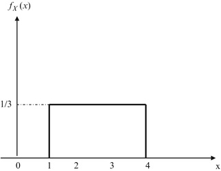
For Prob. 2.27
-
2.28
A continuous random variable X may take any value with equal probability within the interval range 0 to α. Find E[X], E[X2], and Var(X).
-
2.29
A random variable X with mean 3 follows an exponential distribution. (a) Calculate P(X < 1) and P(X > 1.5). (b) Determine λ such that P(X < λ) = 0.2.
-
2.30
A zero-mean Gaussian random variable has a variance of 9. Find a such that P(∣X∣ > a) < 0.01.
-
2.31
A random variable T represents the lifetime of an electronic component. Its PDF is given by
$$ {f}_T(t)=\frac{t}{\alpha^2} \exp \left[-\frac{t^2}{\alpha^2}\right]u(t) $$where α = 103. Find E[T] and Var(T).
-
2.32
A measurement of a noise voltage produces a Gaussian random signal with zero mean and variance 2 × 10⁻¹¹ V2. Find the probability that a sample measurement exceeds 4 μV.
-
2.33
A random variable has triangular PDF as shown Fig. 2.19. Find E[X] and Var(X).
Fig. 2.19 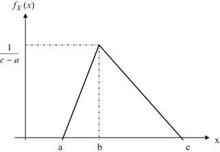
For Prob. 2.33
-
2.34
A transformation between X and Y is defined by Y = e − 3X. Obtain the PDF of Y if:
(a) X is uniformly distributed between −1 and 1, (b) f X (x) = e − x u(x).
-
2.35
If \( {f}_X(x)=\alpha {e}^{-\alpha x,},\begin{array}{cc}\hfill \hfill & \hfill \hfill \end{array}0<x<\infty \) and Y = 1/X, find fY(y).
-
2.36
Let X be a Gaussian random variable with mean μ and variance σ2. (a) Find the PDF of Y = e X. (b) Determine the PDF of Y = X2.
-
2.37
If X and Y are two independent Gaussian random variables each with zero mean and the same variance σ, show that random variable \( R=\sqrt{X^2+{Y}^2} \) has a Rayleigh distribution as shown Fig. 2.20. Hint: The joint PDF is f XY (x,y) = f X (x)f Y (y) and \( {f}_R(r)=\frac{r}{\sigma^2}{e}^{-{r}^2/2{\sigma}^2}u(r) \).
Fig. 2.20 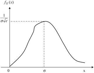
PDF of a Rayleigh random variable for Prob. 2.37
-
2.38
Obtain the generating function for Poisson distribution.
-
2.39
A queueing system has the following probability of being in state n (n = number of customers in the system)
$$ {p}_n=\left(1-\rho \right){\rho}^n,\begin{array}{cc}\hfill \hfill & \hfill n=0,1,2,\cdots \hfill \end{array} $$(a) Find the generating function G(z). (b) Use G(z) to find the mean number of customers in the system.
-
2.40
Use MATLAB to plot the joint PDF of random variables X and Y given by
$$ {f}_{XY}\left(x,y\right)= xy{e}^{-\left({x}^2+{y}^2\right)},\begin{array}{cc}\hfill \hfill & \hfill \hfill \end{array}0<x<\infty, 0<y<\infty $$Limit x and y to (0,4).
-
2.41
Use MATLAB to plot the binomial probabilities
$$ P(k)=\left(\begin{array}{c}\hfill k\hfill \\ {}\hfill n\hfill \end{array}\right){2}^{-k} $$as a function of n for: (a) k = 5, (b) k = 10.
-
2.42
Error in data transmission occurs due to white Gaussian noise. The probability of an error is given by
$$ P=\frac{1}{2}\left[1-\mathrm{erf}(x)\right] $$where x is a measure of the signal-to-noise ratio. Use MATLAB to plot P over 0 < x <1.
-
2.43
Plot the PDF of Gaussian distribution with mean 2 and variance 4 using MATLAB.
-
2.44
Using the MATLAB command rand, one can generate random numbers uniformly distributed on the interval (0,1). Generate 10,000 such numbers and compute the mean and variance. Compare your result with that obtained using E[X] = (a + b)/2 and Var(X) = (b − a)2/12.


Rights and permissions
Copyright information
© 2013 Springer International Publishing Switzerland
About this chapter
Cite this chapter
Sadiku, M.N.O., Musa, S.M. (2013). Probability and Random Variables. In: Performance Analysis of Computer Networks. Springer, Cham. https://doi.org/10.1007/978-3-319-01646-7_2
Download citation
DOI: https://doi.org/10.1007/978-3-319-01646-7_2
Published:
Publisher Name: Springer, Cham
Print ISBN: 978-3-319-01645-0
Online ISBN: 978-3-319-01646-7
eBook Packages: Computer ScienceComputer Science (R0)