Adversarial Logic

Abstract

We introduce Adversarial Logic, an extension of Incorrectness Logic [1] with an explicit Dolev-Yao [2] adversary to statically analyze the severity of security vulnerabilities in the under-approximate setting. Adversarial logic is built on the ability to separate logical facts known to the adversary from facts solely known to the program under analysis. This flavor of program incorrectness can be used to analyze software in which error behavior occurs at deeper levels of interaction between the program and its environment, such as subtle cases of information disclosure requiring multiple program executions to be uncovered. We introduce the Oscillating Bit Protocol, an example algorithm where such a vulnerability can be detected using adversarial logic while remaining elusive to other frameworks. We define a flavor of symbolic execution in which the adversary guides the introduction of symbolic variables and the checking of attack assertions. Additionally, we introduce equivalence testing, an under-approximate version of program equivalence only proven on specific program paths and used to extract differences between comparable implementations. We provide a denotational semantics for adversarial logic and prove its soundness, thereby guaranteeing that extracted attack paths are true positives.

1 Introduction

The ever growing volume of software developed over the last several decades has led to a situation where software vendors and open source projects are unable to keep up with the sheer number of vulnerabilities found and disclosed by the community every year. In just the Linux kernel, a single testing tool [3] identified more than 3,000 bugs in two years, and thousands of others are regularly found in mainstream projects [4]. A crucial problem in the presence of such large numbers of bugs is to determine the practical security implications of each bug to inform which bugs must get fixed first.

Particularly dangerous software attacks attempt to elevate privileges [5] or steal secrets [6] using an adversarial program (or exploit) manually written by a security expert. Determining the potential for compromise of a vulnerable program is a time-consuming task of paramount importance, that has received surprisingly little attention from the formal verification community. This is especially critical as (a) known bugs are left unremediated for a long time, (b) security compromises are increasingly costly and (c) existing tools keep finding hundreds of new bugs every month.

This paper provides a logical foundation for exploit programming [7] dedicated to the static exploitability analysis of program bugs. Not all bugs are considered equal from an exploitability perspective: Can it be used to divert the program’s control flow or corrupt data [8]? Does it allow information disclosure leading to password or private key compromise [6]? Does it allow untrusted code execution as root, or other remote user [5]? Elaborate exploits often require multiple stages of probing the target for reconnaissance [9] or leverage several weak bugs to build a complete attack. For example, an exploit may first attempt to guess internal program addresses using an information disclosure vulnerability to infer the location of sensitive data [10], and then use a subsequent array out of bound access to tamper with said data. Analyzing such bug chaining currently remains out of reach for existing program analysis frameworks.

Historically, program verification has focused on sound and over-approximate analysis guaranteeing the absence of entire classes of bugs in analyzed software [11, 12] at the expense of false positives. To work around program analysis undecidability, recent trends are focusing on under-approximate and complete analyses in which findings are guaranteed to uncover real issues. Theoretical underpinning of bug finding now enjoys a foundational theory of incorrectness logic [1] (IL), a new logic focusing on uncovering true bugs rather than proving the absence of bugs. Fuzz testers [3, 4] and other complete tools are indeed immediately actionable in the software development life-cycle of large software organizations, where the absence of false positives is critical to developer adoption. Incorrectness logic was recently extended to include heap reasoning [13] and concurrency checking [14] demonstrating its versatile nature. Adding an explicit attack program to reason about adversarial behaviors of incorrectness is a fundamentally under-approximate problem, and naturally extends IL.

We introduce adversarial logic (AL), a new under-approximate logic extending incorrectness logic (IL) to determine bug exploitability by leveraging accumulated error in software programs. Adversarial reasoning can be used as a theoretical basis to determine the existence of true attacks in buggy software. The resulting logic gives rise to a notion of attack soundness that captures sufficient conditions for an attack to be guaranteed satisfiable by an adversary. To prove soundness, it is sufficient to demonstrate that some execution paths of the program are exploitable. This differs from typical verification frameworks which attempt to prove statements about all possible program paths. We prove the main attack soundness result of this paper in Sect. 5. AL extends IL in the following ways:

• We consider the system under analysis to be a parallel composition of the analyzed program and an explicit adversarial program attempting to falsify the program specification.

• We focus on proving the satisfiability of anattack contract rather than following the usual methodology of checking code contracts in the program itself.

• We introduce adversarial preconditions, which allows for program errors to accumulate transitively. IL has no error preconditions and only error postconditions.

• We add channel communication rules to model that only explicitly shared program output is visible to an external adversary.

• We introduce a new adversarial consequence rule to derive additional adversarial knowledge otherwise remaining unobserved in program output.

• We generalize the backward variant rule of IL to the parallel case, so that AL can determine the existence of attacks in interactive protocol loops without unrolling the entire attack path.

The new adversarial consequence rule is of particular importance to the discovery of indirect information disclosure attacks, as AL can model leaking of internal program state without assuming its direct observability by the adversary.

It is worth noting that adversarial logic does not encode root cause analysis [15] as it does not attempt winding back to the source of bugs. Rather, it provides a framework to analyze bug effects by considering unintended computations as first-class primitives, allowing the transitive tracking of error conditions through the adversarial interpretation of the program.

The rest of the paper is organized as follow: we introduce a motivating example of an information disclosure attack in the Oscillating Bit Protocol in Sect. 2. We introduce the rules of Adversarial Logic in Sect. 3. We explore additional examples demonstrating the usage of AL in Sect. 4. Among these new examples is a technique to under-approximate program equivalence we call equivalence testing. We give the denotational semantics of AL and prove soundness of AL rules with respect to its semantics in Sect. 5. We briefly provide alternative presentations to adversarial logic based on the formalism of dynamic logic [16] and information systems [17] in Sect. 6. Finally, we cover related work in Sect. 7 and conclude on future work.

2 Motivation

Let us start with an example in Table 1 where an information disclosure attack is performed in $\mathcal {O}(n)$ interactions with the program. Note how the value of the secret variable is used to grant access to the function $do\_serve$. Due to a discrepancy in the return value of the server function, it is possible for an adversary to determine the secret without reading it directly. The server’s observable return value will be 0 (the adversary’s goal encoded in adv_assert on line 14), or 1 (the provided value was too big) or 2 (the provided value was too small). Therefore, an adaptive search can guess the secret value in a maximum attempts of $\mathcal {O}(n)$ instead of the naive brute-force algorithm in $\mathcal {O}(2^n)$ where n is the size of the secret in bits. The oscillating nature of checking the adversarial assertion is represented as a finite state automaton in Table 2.

Table 1. Oscillating bit protocol: target program (Left) and adversary (Right)

Table 2. OBT attack has initial state (I) and started state (S) then oscillates between high (H) and low (L) before terminating in success (T) or failure (F).

Since integer are represented with 8-bits in this example, the adversary would need to consider only 8 + 1 = 9 values before it can successfully guess the secret and satisfy the adversarial assertion. Note that width 8 is chosen for simplicity, and this class of linear-complexity attacks scales very well when x grows to 16, 32, 64, etc. Not all attacks are that simple in practice, and one can imagine polynomial or more complex attack strategies up to infinite ones. The full sequence of interactions in the oscillating bit protocol is given in appendix.

3 Adversarial Logic

Adversarial Logic (AL) marries under-approximate reasoning [1, 18] with an adversarial model [2] suitable for the study of complex software implementation attacks. We will work with this toy imperative language made of variables, expressions, channels, predicates and commands.

Expressions are made of named variables x, concrete integers n, symbolic values $\alpha$, random values, and their arithmetic combinations. Channel variables are named resources ($s_1$, $s_2$, etc.) whose values are ordered lists of scalar values. In particular, the value (s :  : x) is the concatenation of values in channel s with the value of variable x added to the end of s. The value (s$\backslash$x) is the value of channel s after removing the value of x from the head. The value of an empty channel is an empty list.

For simplicity, a small set of scalar variable types T is available, which is sufficient to cover all examples of this paper. Machine encoding of such data types is not central to the logic and remains out of scope for this paper. We will sometimes treat the rand() value as an uint8 (such as the oscillating bit protocol in Table 5) and other times as a float (as in the equivalence testing example of Table 7). We will adopt rand8() or randf() as needed to make precise which version is used, or simply rand() when the version is obvious from context.

Predicates are built from the usual logical and, or, not, as well as equality and inequality tests. All commands can be used in program or adversarial terms, except assertions which are limited to the adversary. The communication primitive Com is distinct from read and write, and Com can be applied at any time after the corresponding write is completed and before the corresponding read is performed. This flexibility makes AL able to encode any desired caching strategy. Although studies of specific caching strategies are out of scope for this paper, attacks leveraging caching behavior are now mainstream [19, 20] and it is critical to allow a spectrum of possibilities as to when communication effectively happens on channels. As such, we leave Com implicit in our examples and apply the corresponding proof rule when required to make progress.

Although AL can reason about the full adversarial term when available, it is not required to be the case and a minimal template is often sufficient. Example 2 and 3 of Sect. 4 show how such templates can be leveraged to build attack proofs. Additional syntactic sugar is defined for convenience purpose:

AL inherits from incorrectness logic in that its semantics is defined using a couple of relations and where is the program interpretation and is the adversarial interpretation. We recall that inference triples in incorrectness logic are written as:

Each code fragment c lifts precondition P to postcondition Q and error postcondition R. We generalize by so that inference triples are written as:

Program interpretation and adversarial interpretation are compositional and allow independent reasoning over and . A novelty of adversarial logic is that assertions are solely checked by the adversary. Rules Success and Failure check the satisfiability of an attack contract rather than a program contract. Checking of assertions augment adversarial knowledge, as both outcomes may inform the choice of subsequent interactions with the program.

More succinctly, rules in AL are written as:

where is a short notation to write two rules c and c as one when the rule is valid in both program and adversarial interpretations. This allows a much more succinct representation of adversarial logic proof rules.

Basic operations such as reading and writing on channels require the use of new Read and Write rules. I/O rules are defined as synchronous primitives, where a read (resp. write) happens immediately if data is available on the (potentially infinite) channel.

Access to channel are implemented using Floyd’s axiom of assignment as applied to channel values (lists). Channels in AL are accessed first-in / first-out and can be used to represent files, sockets, and other inter-process communication primitive of real systems. If an attempt is made to read data on an empty channel, the Skip rule can be used to simulate a blocking read. Reads and writes are performed one datum at a time. Operations on bigger data length can easily be encoded using repetition of these base rules.

Parallel composition of a program $c_p$ and an adversary $c_a$ is constructed from a program interpretation and an adversarial interpretation of parallel terms:

Two parallel terms may either be an adversarial term and a program term, or two independent program terms, with , $\in$ :

The Par rule does not permit communication in itself. This follows from the adversarial logic principle that no information is shared unless explicitly revealed. This parallel rule is unusual as it uses two pre-conditions and two post-conditions, enforcing variable separation without requiring an extra conjunctive connector as done in separation logic [21].

When two parallel terms need to share information, AL requires to use the communication rule Com on channel s. While program and adversary share no local or free variables, shared channels are required for communication. To preserve uniqueness of names, we may use $s_a$ in the adversarial interpretation, and $s_p$ in the program interpretation to refer to channel s, although we will just use s when the meaning is clear from context. Examples of Com usage can be found in the simplest example of next section in Table 3.

Applications of adversarial logic include cases where the adversary wishes to infer hidden values of variables and predicates that have not been communicated. In these cases, the Adversarial Consequence rule can augment the adversarial postcondition $A ^\prime$ if observable values communicated by the program are consequences of hidden program conditions, represented as program predicate Q). We require that $Free(Q) = \emptyset$ as free variables in Q are not defined in the adversarial term. This can be guaranteed by creating fresh names during the introduction of Q in the adversarial context, so that no names are shared. It is assumed that $s \in Chan(A) \cap Chan(P)$. Basic usage of this rule can be found in all examples of Sect. 4.

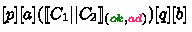
Adversarial logic generalizes the Backward variant rule of incorrectness logic [1] for parallel composition of program and adversarial terms, which we name the Parallel Backward Variant, or PBV.

AL’s backward variant rule is a parallel composition of a program fragment $c_p$ repeated n times with an adversarial code fragment $c_a$ repeated m times. It is not required for the number of program steps n and adversarial steps m to be the same, as long as at least one step is taken at each iteration ($i,j \in \{0,1\} \wedge i + j \ge 1$). This condition enforces that every extracted attack trace is finite. Examples in this article show cases where n = m (the oscillating bit protocol), and others where n $\ne$ m (equivalence testing).

The PBV rule cannot be expressed using two instances of IL’s original BV rule, as PBV can express conditions where adversarial and program conditions are subject to communication. It may also be useful to apply the original sequential BV rule in parallel when program and adversarial terms are independently reducible, however this does not equate to using the parallel version of the rule which can provide synchronization across terms. A practical example of PBV usage is demonstrated in Table 5 of Sect. 4.

One notable incorrectness rule absent from AL is the sequential short-circuit. In this rule, execution of the second term of a sequence is avoided if the first term terminates by an error. As adversarial logic is meant to analyze consequences of erroneous program executions, short-circuiting serves no benefit. This highlights a key difference between IL’s original error relation and AL’s adversarial relation . All other rules of adversarial logic are similar to incorrectness logic with the difference that either or can be used in the precondition, therefore restoring a lost symmetry in incorrectness logic while preserving its meaning.

4 Reasoning with Adversarial Logic

In this section, we put AL to work with three distinct examples. The simplest example of Table 3 is sufficient to explain symbolic variable introduction, adversarial consequence and assertion checking by the adversary. The oscillating bit protocol example from Table 1 of Sect. 2 is then proved step-by-step, including a proof showing the use of the parallel backward variant (PBV) rule for the determination of the existence of attacks. In example 3, two pricing functions are under-approximated to find common price boundaries through adversarial assertions and combines usage of the PBV rule and the adversarial consequence rule to perform equivalence testing.

4.1 Example 1: Trivial Case

Let us consider the example in Table 3 where an adversary wants to capture a flag win with an input value n reaching value 10 million (10M for short).

Table 3. Simple example implementation. The adversary wishes to discover conditions on symbolic variable val to satisfy assertion (res == 1)

Table 4. Simplest example in Adversarial Logic. Unlike traditional program symbolic execution, assertions and symbolic variables can only be introduced in the adversarial part of the system.

An adversarial proof such as the one in Table 4 may contain several proof phases corresponding to non-blocking subsequences of program or adversarial derivations. A proof is typically divided into the following phases:

• 1. The bootstrap phase ($P_0$ to $P_3$ and $A_0$ to $A_3$) where program and adversary have yet to be composed.

• 2. The initial phase ($P_3$, $A_3$) to ($P_9$, $A_9$) typically starts with application of the Par rule until composed terms fail to make more progress other than Skip

• 3. Optionally, one or more intermediate phases separated by applications of the Com rule used to communicate and unblock stuck terms, interleaved with calls to AdvAssert failing to satisfy the attack contract.

• 4. The final phase ends with a call to Success where the adversarial assertion is satisfied ($A_{12}$), or when the adversarial program terminate otherwise.

Note how symbolic variable $\alpha$ is introduced by the adversarial interpretation ($A_1$) and propagated to the program’s logic ($P_4$) using the communication rule. Program and adversarial interpretations remain independent until the parallel rule is used to compose terms. Note how $P_9$ in insufficient to prove the assertion $res == 1$ thus requiring the application of the adversarial consequence rule to obtain additional knowledge $(n = \alpha ) \wedge (n > 10M)$.

4.2 Example 2: Oscillating Bit Protocol

We now analyze the motivating example presented in Sect. 2. It is possible to prove existence of an information disclosure attack in the oscillating bit protocol with or without the parallel backward variant rule. As we will show, use of the PBV rule allows to significantly shorten the proof. Without it, the adversarial interpretation goes through several instances of adversarial failures where $adv\_assert(retcode == 0)$ cannot be satisfied. After a sufficient number of guesses are performed and constraints over the secret are learned, the adversary finally provides a value that matches the secret. In the OBP example, $cred == 160$ is the secret value which cannot be inferred without performing $\mathcal {O}(n)$ steps.

Table 5. Oscillating Bit Protocol (OBT) in AL using disjunction and parallel backward variant rules. Introduction of the PBV rule cut the number of needed steps and can be used to deduce the existence of an attack without guessing the secret.

For brevity, we provide analysis of the example using PBV rule in Table 5, while the version without PBV is given in appendix. A combination of PBV and disjunction rules allows the adversary to find an iteration where the secret is correctly guessed without executing the loop $\mathcal {O}(n)$ times. Recall the form of the PBV rule with $c_p$ the program term and $c_a$ the adversarial term:

In the oscillating bit protocol example, the PBV rule takes a simpler form where n = m and i = j = 1 for all values of (n, m). Applying the PBV rule for this example proceeds as such: P(0) is $secret = v_1$, A(0) is $guess = v_2$, P(n) is $secret = v_1$, A(n) is $guess = v_1$, $P(n+1)$ is $secret = cred$ and $A(n+1)$ is $ret = 0$. Note how P(0) and P(n) are both $s == v_1$ as the secret value does not change across iterations. This condition is not strictly required and may not be guaranteed in more complex examples, such as if the secret variable value changes over time.

We distinguish adversarial proofs which do not appeal to the parallel backward variant rule from those using PBV since the use of PBV allows to reach adversarial success without guessing the secret. Adversarial proofs with PBV are not sufficient to build a concrete attack, but they are sufficient to prove that an attack exists.

4.3 Example 3: Equivalence Testing

Equivalence properties are relevant to security to prove compatibility or indistinguishability of two programs. For example, comparing multiple parsing implementations of a given input language (network headers, ASN.1, etc.) can uncover subtle program behaviors allowing exploitation or fingerprinting of systems [22].

Equivalence results are generally established by showing that the labeled transition system of a program implementation is equivalent to the LTS of its specification [23]. Bisimulation requires two LTS to be observationally equivalent for all transitions. Proving such equivalence is out of reach in the under-approximate framework, in which only some program executions must be analyzed. Take for example the epsilon-delta definition of the limit of a function:

$$\begin{aligned} \forall \epsilon> 0 \exists \delta > 0 : |x - c |< \delta \implies |f(x) - L |< \epsilon \end{aligned}$$

Universary quantified propositions like this one are unprovable in IL and AL, which restricts us to under-approximate equivalence testing for certain inputs. This is useful to prove that two programs are equivalent sometimes, and find values for which programs agree. For $f_1$ and $f_2$ : $\exists x : f_1(x) = f_2(x)$. Let us assume that $f_1(x)$ and $f_2(x)$ can be written as:

$$\begin{aligned}&f_1(x) = \exists x . (P_1(x) \Rightarrow Q_1(x)) \wedge ... \wedge (P_n(x) \Rightarrow Q_n(x)) \\&f_2(x) = \exists x . (R_1(x) \Rightarrow T_1(x)) \wedge ... \wedge (R_m(x) \Rightarrow T_m(x)) \end{aligned}$$

We use this general form where $P_1$ to $P_n$ (resp. $R_1$ to $R_m$) represent the path conditions associated to output values $Q_1$ to $Q_n$ (resp. $T_1$ to $T_m$). Existence of a crossing point between $f_1$ and $f_2$ can now be written as:

$$\begin{aligned} EquTst(f_1,f_2) = \exists x \exists i \exists j : (P_i(x) \Rightarrow Q_i(x)) \wedge (R_j(x) \Rightarrow T_j(x)) \wedge (Q_i(x) \Leftrightarrow T_j(x)) \end{aligned}$$

Testing equivalence of $f_1$ and $f_2$ is computable in adversarial logic even when internal program variables (possibly random ones) are involved in the calculation of $f_1$ or $f_2$. Equivalence testing does not require proving $P_i \Leftrightarrow R_j$ (as required in bisimulation) as internal computations $P_i$ and $R_j$ may be hidden to the adversary. Hence equivalence testing is neither a bisimulation nor a simulation.

Table 6. Two pricing functions with user-supplied order number and random initial price.

Table 7. Equivalence testing: PBV and adversarial consequence rules are combined to find an input for which two pricing functions have the same output.

Consider the code in Table 6 where a pricing service contains two functions GetPrice and GetPrice2 reading on channels $s_1$ and $s_2$ to compute market price based on a globally initialized random market value initp and ordered quantities num. The first function converges faster than the other due to a different current price calculation.

Adversarial logic can be used to prove that functions GetPrice and GetPrice2 meet at the same limit price (a tenth of the initial price) for certain input order quantities above which the price does not decrease anymore. In order to model this example in adversarial logic, we define and use a derived rule Dup at step $(P_2,A_2)$ in Table 7. The Dup rule can be expressed solely based on the parallel rule with parameters and $P_1 = P_2$ and $Q_1 = Q_2$ and $c_1 = c_2$.

The proof exhibits loop iterations at which the price converges, and symbolically compares return values in the adversary. Combining the parallel backward variant rule at $(P_{16},A_{16},Q_{16})$ followed by the adversarial consequence rule at $(P_{17},A_{17},Q_{17})$ gather GetPrice conditions, while this happens at $(P_{28},A_{28},Q_{28})$ and $(P_{29},A_{29},Q_{29})$ for function GetPrice2. This is possible without the adversary having preliminary knowledge of internal program values and state (such as the initial price), as long as the target program code is known.

Table 8. Relational denotational semantics for AL with transitions from state pairs to with and $\varSigma _x \in \{\varSigma _a,\varSigma _p\}$

5 Semantics

In this section, we develop a denotational semantics for adversarial logic. This semantics is defined compositionally for each of the rules of AL (Table 8).

We lay the groundwork to prove soundness of the logic and semantics by reminding some standard definitions.

Definition 1 (Post Image and Semantic Triples)

For any relation $r \in \varSigma \times \varSigma$ and predicate $p \subseteq \varSigma$:

• The post-image of r, $post(r)\in P(\varSigma ) \rightarrow P(\varSigma )$: $post(r)p = \{(\sigma ^\prime \mid \exists \sigma \in p. (\sigma ,\sigma ^\prime ) \in r\}$

• The over-approximate Hoare triple: $\{p\}r\{q\}$ iff $post(r)p \subseteq q$

• The under-approximate incorrectness triple: [p]r[q] is true iff $post(r)p \supseteq q$

We then introduce adversarial semantic triples, which can be understood as a composition of semantic relation between program states $\varSigma _p$ and adversarial states $\varSigma _a$ where $\varPi = \varSigma _p \times \varSigma _a$ is the decomposed view of the state space.

Definition 2 (Adversarial Triples)

For any composed relation and predicates $(p,a) \subseteq \varPi$ with p the program predicate and a the adversarial predicate:

• The post-image of noted :

  

• The under-approximate adversarial triple:

  

Conditions for membership are defined as:

• 1.   and if $VAR(\sigma _p) \cap VAR(\sigma _a) = \emptyset$

• 2.   otherwise.

The first formulation of membership is enough for the Par rule and all rules where program and adversary are reduced independently. The second formulation is needed for the Com, Backward variant and Adversarial consequence rules as a channel s may ve involved to share information between program and adversary.

Definition 3 (Incorrectness Principles in Adversarial Logic)

Adversarial logic preserves the symmetries of incorrectness logic:

• $\wedge \vee$ symmetry:

• $\Uparrow \Downarrow$ symmetry:

Adversarial logic inherits the consequence and disjunction rules of incorrectness logic, and therefore preserves incorrectness symmetries. Under-approximate reasoning is similarly unchanged, preserving principles of agreement and denial [1]. The central tool for soundness proof is the characterization lemma, which relates the state transition system of the denotational semantics to the inference system of adversarial logic.

Lemma 1 (Characterization)

The following statements are equivalent:

• 1.   is true.

• 2. Every state in the conclusion is reachable from a state in the premises:

   

The characterization lemma in Adversarial Logic extends the one of Reverse Hoare Logic of de Vries and Koutavas [18] as inherited by Incorrectness Logic [1]. Sufficient conditions for the characterization lemma to hold can be decomposed into three subcases:

• 1. if  

• 2. if  

• 3. Otherwise: $\forall (\sigma _q,\sigma _b) \in (q,b) \exists (\sigma _p,\sigma _a) \in (p,a)$ :

Cases (1) and (2) yield from the fact that core incorrectness rules of adversarial logic are the same as incorrectness logic. We shall provide additional proofs for rules Read, Write, Success and Failure which are new to AL. Case (3) is necessary when both program and adversary take steps together, as done in parallel composition, communication, backward variant and adversarial consequence rules.

Definition 4 (Interpretation of Specifications)

  is true iff the adversarial triple holds.

Proving that this equivalence holds for AL requires proving the soundness theorem of adversarial logic.

Theorem 1 (Soundness)

Every adversarial logic proof is validated by the rules of adversarial denotational semantics.

To prove soundness, we appeal to the following substitution lemma generalized from reverse hoare logic [18], which we hold true without proving it.

Lemma 2 (Substitution)

$\sigma \in P(n / x) \Longleftrightarrow (\sigma | x \rightarrow n) \in P$. That is:

•   if

•   if

The substitution lemma can be instantiated for the program relation as well as the adversarial relation when $x \in Vars$. There is no ambiguity allowed since AL forbids variable sharing. We also follow de Vries and Koutavas [18] by managing local variables using alpha-renaming, rather than using explicit substitution like O’Hearn [1]. This changes the soundness proof for the local variable rule and the assignment rule. For all symmetric cases involving , we may give the proof one of these two cases and omit the identical proof for the other side.

Proof

We prove soundness for each rule of Adversarial logic. For most cases, we appeal to the characterization lemma of adversarial logic semantics to show that for all post-states of semantic triples, there is a pre-state that satisfies the adversarial precondition of the corresponding rule.

Proof

(Unit). Assume skip and skip . Show that . By skip rule, $P = Q$, so skip is true and . Since and .

Proof

(Constancy). Show that . By induction hypothesis, such that $\sigma \rightarrow \sigma ^\prime$ and . Since $Mod(c) \cap Free(F) = \emptyset$, $\sigma \rightarrow \sigma ^\prime$ preserves F. Therefore .

Proof

(Assume). Let assume B and assume(B) . Show that . Since by assume rule, . By consequence rule, .

Proof

(Rand). Assume x = rand() with . Let and show that . Let us first cover the subcase where and . Take . By the substitution lemma, . By assign rule, . That is, . The second subcase where and can be proved similarly.

Proof

(Assign). Take x = e with . Let and show that . Let us first cover the subcase where . Take . By the substitution lemma, . By assign rule, . Taking we obtain that . The second subcase where and can be proved similarly.

Proof

(Local). Let us first take the case where x . Show that there is . By the substitution lemma, , that is since x is bound. By induction hypothesis and executing backward, we obtain . By the substitution lemma, we have . Since $x \notin Free(P)$, we conclude . The second subcase where can be proved similarly.

Proof

(Read). We first define $\sigma ^\prime = (\sigma | x \mapsto v, s \mapsto l)$ and prove that for all there is By the substitution lemma: That is: By rewriting $s^\prime$, we obtain Executing read backward, we get We can conclude since $\{\sigma | s \mapsto (l{::}v), x \mapsto x^\prime \} \subseteq \{ \sigma | s \mapsto (l{::}v)\}$

Proof

(Write). Let   and write(s,x) . Define $\sigma ^\prime = (\sigma \mid s \mapsto (l{::}v))$ and show that there is a . By the substitution lemma, . That is, . By inlining $s^\prime$ we get . By executing write backward, we obtain .

Proof

(Com). Assume with and $\sigma _1^\prime = (\sigma _1 | s \mapsto l_1)$ and $\sigma _2^\prime = (\sigma _2 | s \mapsto (l_2{::}v))$. Prove for all there exists . By the substitution lemma, . Introducing $s^\prime$, we have By $\llbracket Com(C_1,C_2)\rrbracket$ rule, . Rewriting s using $s^\prime$ we now have: .

Proof

(Iterate). Immediate by semantic definitions and Iterate rules.

Proof

(Sequencing). Immediate by semantic definition and induction hypotheses.

Proof

(Choice). Immediate by semantic definition and induction hypotheses.

Proof

(Disjunction). Immediate by logical definition and $\wedge \vee$ symmetry [1] of AL.

Proof

(Consequence). Immediate by logical definition and $\Uparrow \Downarrow$ symmetry [1] of AL.

Proof

(Par). Immediate by semantic definitions and induction hypotheses.

Proof

(Success). Assume adv_assert(B) by $\uplus$ left subset. Success rule gives us that adv_assert(B) . Show that . Success rule does not modify any variable of , therefore and . Since $(P \wedge B) \Longleftrightarrow P \wedge (P \Rightarrow B)$, we conclude that .

Proof

(Failure). Assume adv_assert(B) by $\uplus$ right subset. Failure rule gives us that adv_assert(B) . Show that . Failure rule does not modify any variable of , therefore and . Since $(P \wedge \lnot B) \Longleftrightarrow P \wedge (P \Rightarrow \lnot B)$, we conclude that .

Proof

(Adversarial Consequence). We know that $(A^\prime \wedge \exists v1 . Q \wedge v1 = v2) \Rightarrow A^\prime$. Applying the consequence rule backwards, implies . Therefore by induction hypothesis, we know . By the second induction hypothesis, we also know that . Applying the parallel rule backward, we obtain that .

Proof

(Parallel Backward Variant). We show that there exists such as and .

Proof

(Case $n = m = 0$). Immediate by definition of Iterate Zero rule, with .

Proof

(Case $n = m$ and $i = j = 1$). By inductive hypothesis, it holds that and there is a $\in$ . We reuse the induction hypothesis several times going backward until we reach

Proof

(Case $n \ne m$). By inductive hypothesis, it holds that . Therefore, . Define $\delta (n,m): (\mathbb {N} \times \mathbb {N}) \rightarrow (\mathbb {B} \times \mathbb {B})$ the function mapping values of (n, m) to their corresponding values $(i_n,j_m)$ where $i,j \in \{0,1\}$. We have three subcases:

• $\delta (n,m) = (0,1)$ and .

• $\delta (n,m) = (1,0)$ and .

• $\delta (n,m) = (1,1)$ and .

Recursively going backward using one of the three subcases, we eventually reach one of the two following termination conditions:

• The program reaches its initial condition before the adversary:

  •   .

  • For all remaining $(m-j)$ steps, we have $\delta (0,m) = (0,1)$

  •  

• The adversary reaches its initial condition before the program:

  •   .

  • For all remaining $n-i$ steps, we have $\delta (n,0) = (1,0)$

  •  

6 Alternative Presentation

Different representations of program semantics can encode much of the same concepts as adversarial logic, albeit at different levels of abstractions. We briefly mention a couple of such representations without deep-diving into their respective theory.

6.1 Dynamic Logic

Many of the concepts put forward in this article can be expressed using the dynamic logic of Harel [16]. Let an adversarial system S = $(W,m,\pi )$ and its specification $\mathbb{A}\mathbb{S} = [f_{s_0}, f_{s_1}, ..., f_{s_n}]$ with $\mathbb {F} \in \mathbb{A}\mathbb{S}$ a list of formulae to be satisfied in order. A structure S can be defined as a triple $(W,m,\pi )$ where W is a non-empty set of states, m is the state transition function, and $\pi$ is a labeling function indicating in which state formulae in $\mathbb {F}$ hold.

$$\begin{aligned} S = (W,m,\pi ) \, \widehat{=} {\left\{ \begin{array}{ll} W = P \times A \\ m: W \rightarrow 2^{W \times W} \\ \pi : F \rightarrow 2^{W} \\ \end{array}\right. } \end{aligned}$$

(1)

Satisfiability $S \vdash \mathbb{A}\mathbb{S}$ can then be defined as conditions on the structure S.

$$\begin{aligned} \exists z s_0,s_1,...,s_n z \widehat{=} {\left\{ \begin{array}{ll} s_0 = (\sigma _{p_0}, \sigma _{a_0}) \in \pi (f_{s_0}) \\ s_n = (\sigma _{p_n}, \sigma _{a_n}) \in \pi (f_{s_n}) \\ \forall j< n : ((\sigma _{p_j}, \sigma _{a_j}), (\sigma _{p_{j+1}}, \sigma _{a_{j+1}})) \in m(p,a) \\ \forall f_k \in \mathbb{A}\mathbb{S} : \exists \, j_1< j_2 < n : \\ - \sigma _{j_1} \notin \pi (f_k) \wedge \sigma _{j_1+1} \in \pi (f_k) \\ - \sigma _{j_2} \notin \pi (f_{k+1}) \wedge \sigma _{j_2+1} \in \pi (f_{k+1}) \\ \end{array}\right. } \end{aligned}$$

(2)

The correspondence between dynamic logic [18] and incorrectness reasoning was remarked by O’Hearn [1]. This correspondence is preserved in adversarial logic with the change that every states is a couple (p, a) representing the product of the program state and the adversary state.

6.2 Information Systems

We now express adversarial logic concepts in the framework of domain theory [17]. In this formalism, we understand adversarial systems as a special kind of Scott’s information system. We define an adversarial system $\mathbb {E} = \{ \mathcal {D}, Con_\mathcal {D}, \vdash , \bot \}$ where $\mathcal {D} = \varPsi _a \times \varSigma \times \varDelta \times \varPsi _p$ is the adversarial domain, $Con_\mathcal {D}$ is the set of all finite subsets of $\mathcal {D}$, $\bot$ is the least informative element of $\mathcal {D}$ and $\vdash$ is an entailment relation on $\mathcal {D}$. The entailment relation operates on a set of contexts $\varPsi _a$, $\varPsi _p$, $\varDelta$, and $\varSigma$, where (Fig. 1 and 2):

• $\varSigma$ is the program input to execute the program with adversarial conditions.

• $\varPsi _p$ is the program context holding the symbolic program P.

• $\varDelta$ is the program output produced by interpreting P with program input.

• $\varPsi _a$ is the adversarial context containing facts known by the adversary.

Fig. 2.

Entailment relations for adversarial systems with $\mathbb {P}$ the program and $\mathbb {A}$ the adversary. $\varSigma$ is the program input, $\varDelta$ is the program output, $\varPsi _a$ is the adversarial context and $\varPsi _p$ is the program context.

Fig. 3.

Expected shape of proof tree in adversarial systems

We distinguish $\varPsi _a$ and $\varPsi _p$ to enforce that program knowledge is not shared to the adversary unless explicitly done so through the $\varPsi _a$ context. Entailment relation $\vdash$ is further partitioned into three sub-relations to distinguish each case of inference:

• $\vdash _\delta : \varSigma \times \varPsi _a \rightarrow \varSigma$ is the adversarial entailment relation.

• $\vdash _\phi : \varSigma \times \varPsi _p \rightarrow \varDelta$ is the program entailment relation.

• $\vdash _\theta : \varDelta \times \varPsi _p \rightarrow \varPsi _a$ is the knowledge entailment relation.

Adversarial entailment $\varSigma \times \varPsi _a \vdash _\delta \varSigma$ derives next symbolic program input based on the previous input and the adversarial knowledge in context $\varPsi _a$. Program entailment $\varSigma \times \varPsi _p \vdash _\phi \varDelta$ allows the program to compute an output value based on adversarial input (or from the program itself in case of recursive or internal procedures). Knowledge entailment $\varDelta \times \varPsi _p \vdash _\theta \varPsi _a$ is the only rule which can increase adversarial knowledge $\varPsi _a$. For example, adversarial knowledge of predicate P(A, B) can be obtained based on an observable program output $C \in \varDelta$ where $\vdash _{\theta } C \implies P(A,B)$ holds with $P(A,B) \in \varPsi _p$, $A \in \varSigma$ and $B \in \varPsi _p$. Reachability on $\mathbb {E}$ is defined as computing the least fixed point of the transitive closure of $\vdash$ to discover if the adversarial specification $\mathbb{A}\mathbb{S}$ is satisfiable. Formally, $\mathcal {D} \vdash \mathbb{A}\mathbb{S} \iff$ $\exists$ $g \in \mathcal {D}$ such as $\{g\} \subseteq lfp _{\mathcal {D}}(\bot _\mathcal {D})$ and $g \vdash \mathbb{A}\mathbb{S}$. The oscillating bit protocol logic can be encoded in formula P as:

$$\begin{aligned} P = (s = 160)&\wedge ((r^n = 0) \Rightarrow (v^n = s)) \wedge ((r^n = 1) \Rightarrow (v^n < s)) \\&\wedge ((r^n = 2) \Rightarrow (v^n > s)) \end{aligned}$$

The initial adversarial term can be encoded in formula $A_0$ as:

$$\begin{aligned} A_0 = (o = 0128)&\wedge (s < v^n \Rightarrow (v^{n+1} = v^n - o^n \wedge o^{n + 1} = o^n / 2)) \\&\wedge (s > v^n \Rightarrow (v^{n+1} = v^n + o^n \wedge o^{n + 1} = o^n / 2)) \end{aligned}$$

Modeling the oscillating bit protocol in this framework is done in appendix.

7 Related Work

Related work in extended static checking and formal verification of software comes with a dense prior art, We enumerate a small fraction of the literature which directly influenced our thinking behind adversarial logic.

Incorrectness logic [1] is used as the starting point to formalize adversarial reasoning. In particular, AL borrows the backward variant rule of incorrectness logic and extend it to the parallel setting, a feature left out of scope of concurrent separation incorrectness logic by Raad et al. [14]. In the other hand, AL drops short-circuiting rules of IL, as program errors in AL must be carried transitively to determine the existence of attack paths. The characterization lemma used in under-approximate reasoning in IL and AL was introduced in reverse Hoare logic [18] and take its root in dynamic Logic [16].

Abstract Interpretation is a program analysis framework pioneered by Cousot and Cousot [12] and considered a reference technique in the verification of the absence of bugs. Abstract interpretation is practical [24] and comes with a rich legacy of applications including the creation of abstractions for theorem proving [25], model checking [26], worst-case execution time analysis [27], thread-modular analysis for concurrent programs [28], and input data tracking [29]. In comparison, adversarial logic (and incorrectness logic before it) cannot guarantee the absence of bugs due to its fundamentally under-approximate nature focused on eliminating false positives at the expense of false negatives. Incorrectness principles have been captured in the abstract interpretation framework by the local completeness logic LCL [30], and algebras of correctness and incorrectness can provide a unified formalism to connect both approaches [31].

Process calculus [23] is a well-established formalism to reason about parallel communicating programs and program equivalence using bisimulation. Abadi and Blanchet [32] designed the spi-calculus to verify secrecy properties of cryptographic protocols in the symbolic model. To the same goal, the proverif [33] tool by Blanchet et al. implements the Dolev-Yao model [2] with explicit attacker. It may be possible to extend proverif to include arithmetic in its specifications language, which is required to implement the examples of this paper.

Separation logic is a well-established logic to encode heap reasoning in program analysis. Separation logic comes in both over-approximate [21] and under-approximate [13] flavors. Combined with parallel constructs, separation logic leads to concurrent separation logics [34] and concurrent incorrectness separation logic [14]. Adversarial Logic provides a limited kind of separation between variables of parallel processes without requiring an explicit separating conjunction. Encoding separation expressiveness without the star operator is not unseen, and was previously implemented in the framework of linear maps [35]. Adding support for heap reasoning is a natural next step for adversarial logic.

Automated bug finding by symbolic execution [36, 37], white-box fuzz testing [38], and extended static checkers [39] using SMT solvers [40] are often used to maximize code coverage in static and dynamic program analysis. These tools typically focus on checking sequential properties of non-interactive parser-like code [41], leaving concurrency out of scope. Symbolic execution using SMT solvers have known scalability issues with path explosions in loops and constraint tracking in deep paths. Adversarial logic addresses these issues by only requiring a subset of paths to be analyzed sufficient to prove the presence of exploitable bugs. AL implements a flavor of concurrent symbolic execution where symbolic variables are introduced by the adversary to drive attack search without requiring knowledge of internal program state. As such, AL can express adversarial symbolic execution [42] as used to detect concurrency-related cache timing leaks.

Automated exploit generation (AEG [43]) leverages preconditioned symbolic execution to craft a sufficient program condition to exploit stack-based buffer overflow security vulnerabilities. Specific domains of heap vulnerabilities for interpreted languages have been demonstrated practical to attack by Heelan et al. [44]. Concepts of adversarial logic could possibly be added to extend AEG, such as for tackling information disclosure vulnerabilities as illustrated by the Oscillating Bit Protocol example in Sect. 2.

8 Conclusion and Future Work

Adversarial logic (AL) is a new under-approximate logic extending incorrectness logic [1] to perform exploitability analysis of software bugs. Reasoning about accumulated error in programs is critical to understand the severity of security issues and prioritize bug fixing accordingly. This new logic can be used to discover attacks which require a deeper level of interaction with the program, such as subtle information disclosure attacks in interactive protocol loops. We provided a denotational semantics and proved the soundness of adversarial logic showing that all exhibited attack traces in AL are true positives. In the future, embedding adversarial logic principles in concurrent incorrectness separation logic [14] will extend adversarial logic with heap reasoning, so AL can also be used to perform exploitability analysis of pointer bugs.

References

O’Hearn, P.W.: Incorrectness logic. Proc. ACM Program. Lang. 4(POPL), 1–32 (2019)
Dolev, D., Yao, A.: On the security of public key protocols. IEEE Trans. Inf. Theory 29(2), 198–208 (1983)
Vyukov, D.: Syzkaller (2015)
Serebryany, K.:Continuous fuzzing with libfuzzer and addresssanitizer. In: 2016 IEEE Cybersecurity Development (SecDev), pp. 157–157. IEEE (2016)
Project, T.A.: Apache log4j security vulnerabilities (2022)
Durumeric, Z., et al.: The matter of heartbleed, pp. 475–488 (2014)
Bratus, S., Locasto, M.E., Patterson, M.L., Sassaman, L., Shubina, A.: Exploit programming: from buffer overflows to weird machines and theory of computation. USENIX; Login 36(6), 13–21 (2011)
Dowd, M.: Sendmail release notes for the crackaddr vulnerability (2003)
Sotirov, A.: Apache OpenSSL heap overflow exploit (2002)
Gruss, D., Lipp, M., Schwarz, M., Fellner, R., Maurice, C., Mangard, S.: KASLR is dead: long live KASLR. In: Bodden, E., Payer, M., Athanasopoulos, E. (eds.) ESSoS 2017. LNCS, vol. 10379, pp. 161–176. Springer, Cham (2017). https://doi.org/10.1007/978-3-319-62105-0_11
Hoare, C.A.R.: An axiomatic basis for computer programming. Commun. ACM 12(10), 576–580 (1969)
Cousot, P., Cousot, R.: Abstract interpretation: a unified lattice model for static analysis of programs by construction or approximation of fixpoints. In: Proceedings of the 4th ACM SIGACT-SIGPLAN Symposium on Principles of Programming Languages, pp. 238–252 (1977)
Raad, A., Berdine, J., Dang, H.-H., Dreyer, D., O’Hearn, P., Villard, J.: Local reasoning about the presence of bugs: incorrectness separation logic. In: Lahiri, S.K., Wang, C. (eds.) CAV 2020. LNCS, vol. 12225, pp. 225–252. Springer, Cham (2020). https://doi.org/10.1007/978-3-030-53291-8_14
Raad, A., Berdine, J., Dreyer, D., O’Hearn, P.W.: Concurrent incorrectness separation logic (2022)
Blazytko, T., et al.: \(\{\)AURORA\(\}\): Statistical crash analysis for automated root cause explanation. In: 29th \(\{\)USENIX\(\}\) Security Symposium (\(\{\)USENIX\(\}\) Security 2020), pp. 235–252 (2020)
Harel, D., et al.: First-order dynamic logic (1979)
Scott, D.S.: Domains for denotational semantics. In: Nielsen, M., Schmidt, E.M. (eds.) ICALP 1982. LNCS, vol. 140, pp. 577–610. Springer, Heidelberg (1982). https://doi.org/10.1007/BFb0012801
de Vries, E., Koutavas, V.: Reverse Hoare logic. In: Barthe, G., Pardo, A., Schneider, G. (eds.) SEFM 2011. LNCS, vol. 7041, pp. 155–171. Springer, Heidelberg (2011). https://doi.org/10.1007/978-3-642-24690-6_12
Kocher, P., et al.: Spectre attacks: exploiting speculative execution. In: 2019 IEEE Symposium on Security and Privacy (SP), pp. 1–19. IEEE (2019)
Lipp, M., et al.: Meltdown. arXiv preprint arXiv:1801.01207 (2018)
Reynolds, J.C.: Separation logic: a logic for shared mutable data structures. In: Proceedings 17th Annual IEEE Symposium on Logic in Computer Science, pp. 55–74. IEEE (2002)
Cardwell, J.R.: Ipv6 security issues in Linux and FreeBSD kernels: a 20-year retrospective (2018)
Milner, R.: Communicating and Mobile Systems: The PI Calculus. Cambridge University Press, Cambridge (1999)
Blanchet, B., et al.: A static analyzer for large safety-critical software. In: Proceedings of the ACM SIGPLAN 2003 Conference on Programming Language Design and Implementation, pp. 196–207 (2003)
Cousot, P., Cousot, R.: Abstract interpretation and application to logic programs. J. Logic Program. 13(2–3), 103–179 (1992)
Cousot, P., Cousot, R.: Refining model checking by abstract interpretation. Autom. Softw. Eng. 6(1), 69–95 (1999)
Wilhelm, R., et al.: The worst-case execution-time problem-overview of methods and survey of tools. ACM Trans. Embed. Comput. Syst. (TECS) 7(3), 1–53 (2008)
Miné, A.: Relational thread-modular static value analysis by abstract interpretation. In: McMillan, K.L., Rival, X. (eds.) VMCAI 2014. LNCS, vol. 8318, pp. 39–58. Springer, Heidelberg (2014). https://doi.org/10.1007/978-3-642-54013-4_3
Urban, C., Müller, P.: An abstract interpretation framework for input data usage. In: Ahmed, A. (ed.) ESOP 2018. LNCS, vol. 10801, pp. 683–710. Springer, Cham (2018). https://doi.org/10.1007/978-3-319-89884-1_24
Bruni, R., Giacobazzi, R., Gori, R., Ranzato, F.: A logic for locally complete abstract interpretations. In: 2021 36th Annual ACM/IEEE Symposium on Logic in Computer Science (LICS), pp. 1–13. IEEE (2021)
Möller, B., O’Hearn, P., Hoare, T.: On algebra of program correctness and incorrectness. In: Fahrenberg, U., Gehrke, M., Santocanale, L., Winter, M. (eds.) RAMiCS 2021. LNCS, vol. 13027, pp. 325–343. Springer, Cham (2021). https://doi.org/10.1007/978-3-030-88701-8_20
Abadi, M., Gordon, A.D.: A calculus for cryptographic protocols: the SPI calculus. Inf. Comput. 148(1), 1–70 (1999)
Blanchet, B., Smyth, B., Cheval, V., Sylvestre, M.: Proverif 2.00: automatic cryptographic protocol verifier, user manual and tutorial, pp. 05–16 (2018)
Brookes, S., O’Hearn, P.W.: Concurrent separation logic. ACM SIGLOG News 3(3), 47–65 (2016)
Lahiri, S.K., Qadeer, S., Walker, D.: Linear maps. In: Proceedings of the 5th ACM Workshop on Programming Languages Meets Program Verification, pp. 3–14 (2011)
Cadar, C., Ganesh, V., Pawlowski, P.M., Dill, D.L., Engler, D.R.: Exe: automatically generating inputs of death. ACM Trans. Inf. Syst. Secur. (TISSEC) 12(2), 1–38 (2008)
Cadar, C., Dunbar, D., Engler, D.R., et al.: Klee: unassisted and automatic generation of high-coverage tests for complex systems programs. In: OSDI, vol. 8, pp. 209–224 (2008)
Godefroid, P., Levin, M.Y., Molnar, D.: Sage: whitebox fuzzing for security testing. Queue 10(1), 20:20–20:27 (2012)
Ball, T., Hackett, B., Lahiri, S.K., Qadeer, S., Vanegue, J.: Towards scalable modular checking of user-defined properties. In: Leavens, G.T., O’Hearn, P., Rajamani, S.K. (eds.) VSTTE 2010. LNCS, vol. 6217, pp. 1–24. Springer, Heidelberg (2010). https://doi.org/10.1007/978-3-642-15057-9_1
de Moura, L., Bjørner, N.: Z3: an efficient SMT solver. In: Ramakrishnan, C.R., Rehof, J. (eds.) TACAS 2008. LNCS, vol. 4963, pp. 337–340. Springer, Heidelberg (2008). https://doi.org/10.1007/978-3-540-78800-3_24
Vanegue, J., Lahiri, S.K.: Towards practical reactive security audit using extended static checkers. In: 2013 IEEE Symposium on Security and Privacy, pp. 33–47. IEEE (2013)
Guo, S., Wu, M., Wang, C.: Adversarial symbolic execution for detecting concurrency-related cache timing leaks. In: Proceedings of the 2018 26th ACM Joint Meeting on European Software Engineering Conference and Symposium on the Foundations of Software Engineering, pp. 377–388 (2018)
Brumley, D., Cha, S.K., Avgerinos, T.: Automated exploit generation. US Patent App. 13/481,248 (2012)
Heelan, S., Melham, T., Kroening, D.: Automatic heap layout manipulation for exploitation, pp. 763–779 (2018)
Acknowledgments
The author thanks Peter O’Hearn, Azalea Raad and Samantha Gottlieb for their useful reviews of this paper.
Author information
Authors and Affiliations
Corresponding author
Editor information
Editors and Affiliations
Rights and permissions
Copyright information
© 2022 The Author(s), under exclusive license to Springer Nature Switzerland AG
About this paper
Cite this paper
Vanegue, J. (2022). Adversarial Logic. In: Singh, G., Urban, C. (eds) Static Analysis. SAS 2022. Lecture Notes in Computer Science, vol 13790. Springer, Cham. https://doi.org/10.1007/978-3-031-22308-2_19
Download citation
DOI: https://doi.org/10.1007/978-3-031-22308-2_19
Published:
Publisher Name: Springer, Cham
Print ISBN: 978-3-031-22307-5
Online ISBN: 978-3-031-22308-2
eBook Packages: Computer ScienceComputer Science (R0)