Fundamentals of Groundwater Modeling Methods and a Focused Review on the Groundwater Models of the Nile Valley Aquifer

Abstract

Groundwater plays an essential role in the overall management of water resources. The demand for groundwater for municipal, agricultural, and industrial use has been grown steadily during the past decades. Groundwater modeling can be used to evaluate the quantity and quality of groundwater in aquifer-aquitard systems, also in relation to environment and climate change. Modeling allows for the construction of scenarios based on different groundwater abstraction rates, changes in human activities, and varying environmental conditions. Models can be based on simple analytical methods and comprehensive finite difference or finite element methods, dependent on the model’s purpose and the available data. Conceptualization and data collection strongly influences the choice of the numerical model. In the past finite difference and finite element methods were considered as completely different, but more recent developments closed the gap between these two methods. Generally, the time-independent data like spatially distributed hydraulic conductivities, etc. are not available at the start of the modeling. These parameters have to be determined from a time series of both measured and calculated quantities, for instance hydraulic heads, This process is generally called model calibration, or parameter estimation. Groundwater modeling is intending to represents reality in a simplified form, without making too simple assumptions for the purpose of the modeling study; for instance scenarios to investigate the response of an aquifer-aquitard system for a number of hypothetical phenomena like, for instance flash rains or excessive droughts. Several numerical groundwater flow models have been developed for different parts of the Nile Valley aquifer to assess the interaction between the surface water and the aquifer, to apply various management recharge and discharge scenarios. All studies have shown that groundwater modeling can be used successfully to help understand the Nile Valley aquifer's behavior.

1 Background

Groundwater is of great importance in securing most water needs in several regions worldwide (Suring 2020). Many ambitious water resources plans in developing countries are based on the groundwater for achieving the targeted agricultural expansion for the increase of population. Switzerland, Romania, Hungary, Denmark, Belgium, and Austria are examples of such countries where groundwater resources exceed 70% of the total water consumption (Nriagu 2019). Groundwater resources are not independent while they represent a substantial element in the hydrological cycle. Therefore, groundwater is in continuous interaction with the surrounding water bodies and environment. It is also being affected by most of the changes in natural processes, land uses, and field conditions [e.g., agricultural practices (Awad et al. 2021), human activities, and urbanization (Zhao et al. 2013)]. The condition of a particular groundwater resource much depends on these interactions. Thus the best management of groundwater resources is that which considers, as much as possible, all parameters and interactions that can affect the groundwater (Zhou and Li 2011).

The most known and direct technique to assess a particular groundwater resource is through observational works. Particularly, groundwater tables and quality at the targeted domain or area can be monitored at the desired timeframe and time intervals, similar in the study Awad et al. (2020). While such observations cannot answer some questions about, for example, the long-term hydrologic responses of groundwater resources to some significant environmental phenomena, human activities, and even future climate changes. Therefore, groundwater models were developed to play an essential role in facilitating the consideration of different impacts of climate, environmental, and human conditions on groundwater resources, thus improving and enhancing groundwater management (Zhou and Li 2011; Kumar 2019). Groundwater modeling has been practiced around the world to fulfill the following:

• Simulation and analysis of various responses of the groundwater to the surrounding environmental conditions.

• Investigating and understanding different groundwater dynamics and flow patterns.

• Evaluating the various aquifers' processes of recharge, discharge, and storage.

• Predicting future impacts of human activities and climate changes on groundwater resources.

• Planning the collected field data and designing practical solutions for groundwater issues.

Therefore, groundwater modeling is considered a visualization tool through which key messages about groundwater resources can be communicated to the public and decision-makers. Many researchers around the worlds used groundwater modeling to fulfill, and not limited to, the following:

• Assessment of potential impacts of climate change on aquifers (Al-Maktoumi et al. 2018).

• Assessment of the efficiency of groundwater replenishment through natural reservoirs (Salem et al. 2020).

• Investigate the role of chemical fertilizers and pesticides in groundwater contamination (Srivastav 2020; Eltarabily et al. 2017).

• Assessment of how aquifers' conditions can be impacted under different groundwater extraction scenarios (Al-Maktoumi et al. 2016, 2020; El-Rawy et al. 2019a; Eltarabily et al. 2018; Negm 2018).

• Understanding the mechanism of groundwater and surface water interactions (Fleckenstein et al. 2010; Dawoud and Ismail 2013; El-Rawy et al. 2016, 2021a, 2021b).

Tian et al. (2015) coupled groundwater and surface water flow model (GSFLOW) with storm water management model to study the groundwater system along with the hydrologic cycle in the Zhangye Basin, northwest China. Polomčić and Bajić (2015) used the groundwater modeling to decide the best scenario of the dewatering process in the Buvač open cast mine, Bosnia and Herzegovina. Nagels et al. (2015) built a transient groundwater flow model to dewater the groundwater levels in the Schietveld region of Belgium and studied the relationship between hydrology and vegetation types' spatial distribution. Attard et al. (2016) developed a 3-D heat transport modeling approach to quantify underground structures' impact on urban groundwater temperature in the greater Lyon area, France. El-Rawy et al. developed a numerical groundwater flow model for the Zarqa River Basin (Jordan) to predict changes in the aquifer and Zarqa River under different recharge rate scenarios from the As Samra wastewater treatment plant (WWTP) and different groundwater pumping rates. The MODFLOW model was used by Sashikkumar et al. (2017) found suitable areas for artificial recharge structures to boost groundwater supplies in the Kodaganar river basin, Dindigul district, Tamil Nadu. They evaluated its effectiveness using a combination of GIS and numerical groundwater modeling tools. Bishop et al. (2017) explored groundwater pathways, recharge heights, and nitrate sources on Maui, Hawaii, using numerical groundwater modeling. Al-Maktoumi et al. (2018) evaluated the impacts of climate change and the rise of the sea level on Oman's Samail and Jamma coastal aquifers numerically using MODFLOW and MT3DMS. Salem et al. (2018) developed a 3-D groundwater model using MODFLOW-2005 for the Drava floodplain, Hungry, for better understanding the Drava floodplain system's water budget under different lake replenishment scenarios.

El-Rawy et al. (2020a) developed analytical and numerical groundwater flow solutions for the femme-modeling environment in order to examine the effects of rising Aa River water levels on the groundwater aquifer in the Nete River watershed, Belgium. Katpatal et al. (2021) used the GIS and MODFLOW model to simulate future groundwater scenarios in Maharashtra, India, to overcome the drastic decrease in groundwater levels in the study area. The MODFLOW and RT3D models were used by Esfahani et al. (2021) to simulate diffusion and reaction in aquifers without discretizing low permeability zones. Zijl and El-Rawy (2019) studied the evolution from a steady to a steady mixing zone between two groundwater flow systems with varying concentrations. Kenda et al. (2018) implemented machine learning methodologies to model the changes in groundwater levels in the Ljubljana polje aquifer, Slovenia. Meredith and Blais (2019) constructed a groundwater model in the alluvial gravel aquifer of the Bighorn River Valley north of Hardin, Montana, to quantify groundwater recharge's relative importance infiltration of flood-applied irrigation water versus leakage from irrigation canals. Sathe and Mahanta (2019) used the numerical groundwater modeling software to develop a 3-D transient state predictive (groundwater flow and contaminant transport) conceptual model for two arsenic-contaminated regions, to evaluate the groundwater flow and arsenic contaminant transport. An adaptive neuro-fuzzy inference system was trained and optimized by Kisi et al. (2019) to model groundwater quality variables in Iran. El-Rawy et al. (2019a) and Al-Maktoumi et al. (2020) used MODFLOW to develop a groundwater flow and transport model to explore the feasibility of managed aquifer recharge (MAR) utilizing treated wastewater (TWW) in the Jamma coastal aquifer and Al-Khod aquifer in Oman. Zijl and El-Rawy (2021) studied the relevance of the deep creep flow of the earth’s viscous upper mantle and crust as a complement to the groundwater flow. Rahnama et al. (2020) applied the Groundwater Modeling System (GMS) software and MODFLOW model to study the variations in groundwater levels in Shahdad Aquifer, Iran. Another groundwater model was developed by Khadim et al. (2020) using the MODFLOW-NWT in the Gilgel-Abay Catchment, Upper Blue Nile, Ethiopia, where there is data scarcity. They proposed an approach that can combine different types of datasets (e.g., reanalysis products, satellite data, citizen science data, etc.) to overcome the data-scarce issue. To alleviate water shortage difficulties in the Drava River floodplain, Salem et al. (2020) created a combined surface water (Wetspass-M) and groundwater (MODFLOW-NWT) model.

This chapter presents a review of groundwater flow models’ fundamentals, including the boundary conditions, calibration methods, validation, sensitivity analysis, model uncertainties, and limitations of numerical modeling techniques; in this context attention is paid to more recent developments closed the gap between the finite difference and the finite element method. In addition, this chapter presents a review of the groundwater modeling applications on the Nile Valley aquifer in Egypt.

2 Groundwater Modeling

2.1 Introduction

Groundwater resources are essential for sustainable demographic and economic growth (Gleeson et al. 2012). Groundwater modeling is the way of representing reality, in a simplified form without making invalid assumptions or compromising the accuracy, to investigate the system response under certain phenomena or predict the system's behavior (Baalousha 2008). Groundwater models are a powerful tool for efficient management and planning of water resources, groundwater remediation, and protection. In general, models are conceptually describing the approximated physical systems using mathematical equations (Kumar 2004). A better understanding of the physical systems and the embedded assumptions in the mathematical equations are required to assess the usefulness or applicability of the model. These assumptions include the fluid dynamics, the anisotropy and heterogeneity of the bedrock or sediments within the aquifer, aquifer geometry, chemical reactions, and the contaminant transport mechanisms. Models should be considered as an approximation not as an exact representation of reality because of the uncertainties in the model's data and the assumptions embedded in the mathematical equations. Figure 1 shows the main steps of methodology in groundwater modeling. The first step in the modeling process is defining the model's purpose. Data collection represents a significant issue in the modeling process. The model's conceptualization is the fundamental step in modeling, followed by setting up the numerical model. Model calibration and validation, and sensitivity analysis can be performed after model completion. The last step is preparing and running simulations for prediction scenarios.

Fig. 1

A schematic stepwise diagram of groundwater modeling methodology

2.2 Defining the model’s Objectives

The modeling approach, including the choice of model type, may vary depending on the modeling objectives. Groundwater models can be applied as predictive, interpretive, or generic tools (Anderson and Woessner 1992a, b). Predictive models are used to predict the effects of a proposed action on existing hydrogeologic conditions or to assess the future change in groundwater heads, flow rate, or solute concentration. Interpretive models are applied to investigate a particular case, study system dynamics, and evaluate groundwater flow or contaminant transport. Generic models are used to assess different scenarios of remediation schemes or management of water resource and identify regions' suitability for some proposed action. Note that calibration is a prerequisite for predictive models, whereas calibration is not required for interpretive and generic models. Baalousha (2008) summarized the objectives of groundwater modeling as:

• Predicting the temporal and spatial distribution of groundwater head and flow rate.

• Assessing the impcats of groundwater extraction on the flow regime and predicting the resulting drawdown.

• Evaluating the impact of human activities (e.g. agricultural activities, wastewater discharge, landfills, etc.) on groundwater quality.

• Investigating the effect of implementing various management scenarios quantitatively and qualitatively on groundwater systems.

2.3 Conceptual Model

A conceptual model represents the most important part of groundwater modeling; it is built on understanding how a groundwater system works. It consists of understanding the groundwater system’s characteristics and spatio-temporal evaluation and provides a descriptive representation of the hydrogeologic system. Conceptualizing the groundwater system requires good information about hydrology, geology, hydraulic parameters, and boundary conditions. A good conceptual model should simplify the complexity of reality to achieve management requirements and modeling objectives (Bear and Verruijt 1987). Simplification relies on the objectives, the amount of available data, the scale of the model, and the current understanding level. The conceptual model describes factors that include:

• Model domain and aquifer geometry

• Time-independent aquifer/aquitard parameters such as hydraulic conductivity, hydraulic resistance, transmissibility, porosity, specific yield (effective porosity), specific storage, etc.

• Boundary geometry and boundary conditions

• Evapotranspiration and groundwater recharge

• Identification of sources and sinks

• Water balance.

The model's conceptualization is an iterative process that can identify the data gaps which have to be filled by further data gathering for model improvement. Remote sensing data can be used in building the conceptual model, particularly in situations of data scarcity where data-bases and maps may not be adequate. Hydrogeological data should be reliable and sufficient to some extent based on the targeted accuracy level to construct a proper conceptual model.

2.3.1 Boundary Conditions

Defining model boundaries represents the most critical step in building a reliable and accurate numerical groundwater model (Franke et al. 1987). The boundaries and the conditions that have to be applied as boundary conditions are strongly dependent on the hydrogeological conditions in the model domain. To achieve adequate conditions, the following inputs are used:

• (i) Surface data and information from different available maps (topographic, hydrogeological, geological, soil, etc.) and remote sensing images for defining spatial distribution of impermeable lithological contacts, groundwater discharge zones, surface water bodies (river, an artificial reservoir, pond, canal, etc.), springs, geological faults, etc. These surface data can help in defining the recharge or no-flow boundaries (Singhal and Gupta 2010).

• (ii) Subsurface data and information based on boreholes, geophysical surveys, geological sections, etc. These are used for defining subsurface hydrogeological characteristics such as the thickness of different aquifers and aquitards, weathering depths, subsurface salinity variations, buried channels, faults in basement rocks, etc.. Specifying boundary conditions is required to solve groundwater flow equations and represents the first step in model conceptualization. Improper representation of boundary conditions influence the solution and leads to incorrect results. Boundary conditions can be classified into three main types:

  • (a) Type I boundary, called Dirichlet condition, represents specified head.

  • (b) Type II boundary, called Neumann condition, represents specified flow rate.

  • (c) Type III boundary, called Cauchy condition, represents head-dependent flow rate.

In particular, the following types of boundaries are described:

• Constant head boundary: This is a subset of the specified head boundary in which the head or concentration remains constant over time.

• Specified head boundary: This is a generalization of the constant head boundary, which has to be imposed when head or concentration can be identified as a function of location and time. Rivers and streams represent examples of the specified head boundary.

• No flow boundary: This is a special form of a specified flow or flux boundary. It has to be imposed at a surface where the normal component of the flux equals zero. Examples are: the impervious base of the basin (aquifer/aquitard system), groundwater divides, impermeable subsurface layers, and impermeable faults (see Fig. 2).

  Fig. 2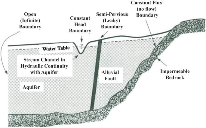

  

  Source Roscoe Moss Company (1990). http://ecoursesonline.iasri.res.in/mod/page/view.php?id=1852

  Typical model boundary conditions

• Specified flux boundary: This is a generalized form of the no-flow boundary. This condition has to be imposed on the boundaries where the normal component of the flow rate (flux) is known as a function of location and time. For instance, it describes spring flow, measured flow from surface water bodies, and seepage to and from bedrock underlying the aquifer/aquitard system.

• Head-dependent flux boundary: This condition has to be imposed on boundaries through which the flux depends the head neighboringto that boundary. A semi-confined aquifer is one in which the water head is determined by the flux through the semi-constricting layer and semi-permeable or leaky faults (Fig. 2). It shows examples of these types of boundaries.

Strictly speaking, there is a fourth type of boundary condition that does not correspond with the Dirichlet, Neuman or Cauchy types. The water table (Fig. 2) or phreatic surface, which is the top boundary of the groundwater model domain, is a moving boundary, going up and down during the seasons, rising during rainfall and falling in drought periods. On that case, two additional types of boundary conditions have to be imposed: a kinematic condition and a dynamic condition. Although the character of this top boundary is often overlooked, it is important to consider its conceptual consequences in more details. The kinematic boundary condition describes the evolution in time of the water table height, function H(x, y, t), with respect to vertical height z, (Strictly speaking, there is a fourth boundary, namely the water table or phreatic surface, which is the top boundary of the groundwater model domain. It is a moving boundary, going up and down during the seasons, rising during rainfall and falling in drought periods. On that boundary two boundary conditions have to be imposed, a kinematic condition and a dynamic condition. Although this top boundary is often overlooked, it is important to consider its conceptual consequences. Strictly speaking, there is a fourth boundary, namely the water table or phreatic surface, which is the top boundary of the groundwater model domain. It is a moving boundary, going up and down during the seasons, rising during rainfall and falling in drought periods. On that boundary two boundary conditions have to be imposed, a kinematic condition and a dynamic condition. Although this top boundary is often overlooked, it is important to consider its conceptual consequences.

The kinematic condition describes the evolution in time, t, of the water table height, H, with respect to the vertical coordinate, z. That is, z = H(x, y, t) in which x and y are the horizontal coordinates. In this condition the specific yield (a parameter) and the recharge rate (a flux condition) have to be specified. It is important to note that water table height H is only a function of the horizontal coordinates and of time; H is independent from the vertical coordinate.

The dynamic condition is essentially the condition that on the water table the groundwater pressure is equal to the atmospheric pressure. The hydraulic head (briefly, the head) is essentially defined as the difference between actual pressure and hydrostatic pressure; this pressure difference is scaled in such a way that it is expressed as a height, head h(x, y, z, t), a function of the horizontal and vertical coordinates as well as time,. The dynamic condition can then be written as h(x, y, z = H, t) = H(x, y, t).

Only under the assumption that in the phreatic aquifer head h is independent from vertical coordinaten z it is possible—but not desirable—to equate the functions h and H. This assumption is known under the name Dupuit approximation. However, when dealing with general three-dimensional flow problems—for instance when dealing with Thótian flow systems—it is necessary to make a clear distiction between head h and height H in order to avoid serious mistakes. For more details see De Smedt and Zijl (2018) and Zijl and Nawalany (1993); also see Sect. 2.10.1.

2.4 Types of Models

There are several types of models available to model groundwater flow and contaminant transport. Models can be divided into three types: physical, analog, and mathematical.

2.4.1 Physical Models

Physical models such as sand tanks rely on developing the models in the laboratory to investigate specific contaminant transport or groundwater flow problems. Using these models, different hydrogeological phenomena such as artesian flow or the cone of depression can be investigated. In addition to flow, contaminant transport can be evaluated through physical models. Such models are easy to set-up and useful; however, they cannot be used to investigate complicated realistic problems.

2.4.2 Analog Models

The flow of electricity represents the most famous analog model. The electric analog depends on the similarity between Darcy’s law relating head difference to groundwater flow rate and Ohm’s law relating potential difference to electric current. Simple analog models can be set up easily to evaluate the groundwater flow. A detailed description of analog models can be found in (Anderson and Woessner 1992a, b; Fetter 2001).

2.4.3 Mathematical Models

Mathematical models represent a conceptual understanding of the groundwater system through a set of partial differential equations describing the flow and transport in the modeling domain where the equations are complemented with initial and boundary conditions. In addition, these equations require specification of spatially distributed time-independent parameters like hydraulic conductivity, storage coefficient, specific yield, porosity, etc., briefly the physical characteristics of the subsurface (aquifer/aquitard system). If both the time-independent pareameters (conductivities, resistances, etc.) and the time-dependent boundary conditions (recharge rates, well abstraction rates, etc.) are specified, the time-evolution of the heads and velocities can be determined from the mathematical model. This so-called forward model can be solved analytically in case of simple systems, or numerically in more complex systems.

2.5 Solution of Mathematical Formulation

As discussed in the preceding sections, the resulting equations of the mathematical model can be solved analytically in case of a simple system, or numerically in more complex systems. Some techniques use a mixture of analytical and numerical solutions.

2.5.1 Analytical Solutions

The primary benefits of using analytical solutions are that they are simple to implement and provide accurate and consistent results for simple problems. Because analytical solutions require many assumptions and simplifications, such as the homogeneity of a simple aquifer/aquitard sequence, they cannot handle a variety groundwater systems and are limited to simple ones. Some examples of analytical solutions include the Theis equation (Theis 1941) and Tóth's solution (Tóth 1962). Bear (1979) and Walton (1989) provide more information on analytical solutions to groundwater problems (1989). Darcy’s law, in the form of its initial form, is the simplest equation describing groundwater flow. In this simplest form, Darcy’s law is used to calculate one-dimensional groundwater flow through a section of an aquifer (Driscoll 1986):

$$Q= \frac{K A ({h}_{1}- {h}_{2} )}{L}$$

(1)

where, Q is the flow rate (m³/day), K is the hydraulic conductivity averaged over the length of the one-dimensional section of the aquifer (m/day), A is the area (m²), ${h}_{1}- {h}_{2}$ is difference in hydraulic head (m), L is the distance along the flowpath between the points, where ${h}_{1}$ and ${h}_{2}$ are measured (m). For the generalization of Darcy’s law to two- and three-dimensional flow see Delleur 2006, Cushman and Tartakovsky (2016), and De Smedt and Zijl (2018).

2.5.2 Numerical Solutions

Numerical methods have been developed to overcome the limitations of analytical solution methods and to deal with the complexity of groundwater systems. Numerical models are based on numerical solutions of a system of coupled algebraic equations for discrete variables, e.g. heads in the nodal points of a discretized flow model, or solute concentrations in the nodes of a discretized transport model. Numerical groundwater models are generally based on the discretization of a model area into a great number of finite volume elements, in such a way that the fundamental conservation laws of mass, momentum and energy are honored for each volume element (Hölting and Coldewey 2019). Several types of numerical solution methods are available for groundwater flow and transport studies. Generally speaking, a distinction can be made between two types of approach: (i) the Finite Difference Method (FDM) and the related Finite Volume Method (FVM) and (ii) the Finite Element Method (FEM).

The Boundary Element Method (BEM) and Analytical Element Method (AEM) (Strack 1989) are based on analytical solutions combined with some form of disctetization—mainly discretization of the boundaries—and therefore result in a system of algebraic equations that has to be solved numerically. The advantage of BEM and AEM is that the flow around the wells can be solved very accurately because there is no need for grid refinement as required for FDM/FVM and FEM. On the other hand, FDM/FVM and FEM can easily handle all types of heterogeneity. For that reason FDM/FVM and FEM are generally considered as the most flexible types of numerical models (Anderson and Woessner 1992a, b; Igboekwe et al. 2008) and are therefore the most widely applied numerical methods. In summary: both in FDM/FVM and FEM, the subsurface is discretized (sub-divided) into a grid with a great many of small finite volumes. The heads and concentrations are calculated in nodal points, while the flow rates have to be considered at the grid faces between the grid volumes in order to analyze the flows through the subsurface (the aquifer/aquitard) system (Igboekwe and Achi 2011).

2.5.2.1 Finite Difference Methods

FDM has been widespread used in groundwater studies since the early 1960s. The finite difference method was alreadty studied by Gauss, Newton, Laplace and Bessel (Pinder and Gray 1977). The basic principle of FDM is to represent the derivative of the head function approximately at discrete points situated between adjacent head values near that point; in other words, derivatives are approximated by difference quotients. The distribution of nodes in FDM is regular (rectangular blocks) but the nodal spacing may either be uniform or non-uniform along the orthogonal coordinate system (Singhal and Gupta 2010). The accuracy of the FDM relies on grid size and uniformity. The approximation of the derivative improves as the grid spacing becomes smaller and smaller, and in the limit of zero grid spacing the numerical approximation becomes equal to the exact solution. For larger grid spacing the solution will deviate more from the exact solution. However, in the calculation of heads and velocities, even if they are relative inaccurate because of a coarse discretization, the mass balance will be honored accuurately provided that the system of algebraic equations is solved with sufficient accuracy. On the other hand, in transport models a coarse discretization gives rise to much larger numerical dispersion than the real physical dispersion. There are different approaches to finite difference approximations: the three most extreme forms are (i) central differences, (ii) forward differences, and (iii) backward diffrences.

In theory central differences provide the best results because in that case the truncation error has a second-order accuracy (∆x)² (Pinder and Gray 1970). However, in the most practical, and therefore most popular finite difference method—the block centered finite difference method—deviatins from the central differences are generally accepted because the rate of convergence to the exact solution does not apprecially deviate from the second-order convergence accuracy (∆x)². This result has been proved by Weiser and Wheeler (1988) (also see the discussion on the’face-centered finite element method’ in Sect. 2.5.2.2). Irregular spacing is often needed to increase the accuracy at selected areas, especially near wells. As a rule of thumb for refining or expanding the finite-difference grid, the maximum multiplication factor should be 1.5 or smaller (Soderlind and Arevalo 2017). Local grid refinement, for instance around each individual well in a flow field, is not possible in finite difference grids. The best approach would be to apply around each well a refined tetrahedral grid (in 3D) or triangular grid (in 2D) in combination with the’face-centered finite element method’; see Sect. 2.5.2.2. However, for practical reasons application of a simple algebraic model relating grid block head to well head is generally used (see, for instance, Peaceman 1978).

The main advantage of the FDM, and in particular of the block-centered FDM, is the flux continuity, which means that the groundwater velocities are continuous at the faces between two adjacent grid blocks. Flux continuity is a prerequisite to obtain accurate solutions of transport problems and/or flow path tracking. In this sense finite difference methods are superior above conventional finite element methods (see Sect. 2.5.2.2). On the other hand, flux continuous methods are not head-continuous. The heads are continuous only in the centers of the grid faces, at the other locations of the faces the heads’jump’ between two neighboring grid blocks. This is in contrast to conventional finite element methods, who are head-continuous. Another contrast is that the FDM under estimates the values of the hydraulic conductivities, while the conventional finite element method over estimates them.

The available finite difference models are easy to implement, well documented and proven to provide good results. The main disadvantage is that these methods do not fit properly to an irregular model boundary. Moreover, the grid's size (number of grid blocks) highly influences the computational effort and accuracy. MODFLOW is the most commonly used finite-difference groundwater model (Harbaugh and McDonald 1996).

2.5.2.2 Finite Element Methods

In the finite element method (FEM), the model domain is divided into many relatively small sub-regions, the volume elements (briefly the elements), which may have any shape. In each element head and velocity are represented by a relatively simple algebraic function of the spatial coordinates In addition, the FEM can handle any type of anisotropy including hydraulic conductivity tensors with off-diagonal components. In the FEM, the integral representation of a partial differential equation is obtained by one of the following approaches: variational principle, weighted residuals, or Galerkin’s method. A detailed description of these method can be found in Pinder and Gray (1970). As the FEM uses irregular shapes of the elements, the nodes of the elements can be scattered arbitrarily in the domain, in concentrated or sparse patterns, to form various sizes of elements. This flexibility of the finite element grid enables a more realistic simulation of different boundaries (Singhal and Gupta 2010) and is useful for providing a close spatial approximation of irregular boundaries and for concentrating elements in areas where the considered variable is characterized by larger variations and where higher accuracy is required (Bear and Cheng 2010). Especially when dealing with grid refinement around wells, these advantages play a major role.

FEM requires more sophisticated mathematics and may provide more accurate results for a number of applications. The conventional finite element method is head-continuous over the faces (face elements) between two adjacent volumes (volume elements), which makes the method very suitable for soil-mechanical and geo-mechanical problems. However, because the conventional finite element method is not flux continuous, the conventional FEM is not suitable for transport problems, in contrast to volume centered finite difference methods.

A notable exception is the’face centered’ finite element method (in mathematical terms: the’mixed-hybrid finite element method’). In this method the heads are calculated in the centers of the faces and are discontinous at the other points of the faces (in mathematical terms the face-centered heads are the’Lagrange multipliers’). The face centered finite element method is flux continuous and, therefore, suitable for transport problems. Grid refinement results in good convergenge to the exact solution The face-centered finite element method is algorithmically different from the block centered finite difference method (e.g. MODFLOW), but when refining the finite diference grid of the block centered finite difference method, this method converges in the same way to the solution obtained by the face-centered finite element method (Weiser and Wheeler 1988). Thanks to this result the modeling community has fully accepted the block centered finite difference method. It has good convergence properties; therefore there is no longer a reason to use the more complex point distributed finite difference method (Azis and Settari 1979, Sect. 3.5.1). In contrast to the conventional finite element method, the face centered method is under estimating the hydraulic conductivities. For more details about the face-centered finite element method or, in mathematicl languege, mixed-hybrid finite element method see the’pioneers’ Chavent and Jaffré (1986) and Kaasschieter (1990), Kaasschieter and Huijben (1992); they applied and exempified the face-centerd finite element method for petroleum reservoir engineering and groundwater flow modeling, respectively.

Unfortunately, the highly mathematical presentation of this method has seriously hampered its understanding and acceptance by the hydrogeological community. Fortunately, Bossavit (1998, 2005) was able to present an alternative, much more transparant approach to replace the opaque mathematics and its terminology. Although Bossavit presented his theory in the context of electrical engineering, his approach could relatively easily be translated to groundwater flow; Trykozko (2001), Trykozko et al. (2001), Zijl (2005a; b).

In the finite element method the identification and construction of the input data set is more complicated than for a regular finite difference grid. Mesh design in the finite element method is crucial as it significantly influences the accuracy and convergence of the solution. It is highly recommended to keep the mesh configuration simple and to refine the mesh only at interesting areas where variables change rapidly, in particular near sources and sinks. It is better to keep the mesh configuration as simple as possible. To facilitate the construction of a finite element mesh it almost necessary to to use a pre- and post-processor. For further details on the use of FEM modeling, the reader is referred to Remson et al. (1971), Pinder and Gray (1977), and Huyakorn and Pinder (1983). The most common finite element based groundwater models are MODFE (Torak 1993), Femwater (Lin et al. 1997), and FEFLOW (Wasy 2005).

2.6 Model Calibration

The objective of calibration is to determine the time-independent parameters in the model; for instance the spatially distributed of hydraulic conductivities. This is achieved by feeding the model with input data, generally a time series of flow rates (of recharge rates, well rates, etc.) and comparing the computed output variables to the measured time-dependent heads, flow rates and concentrations with the values measured in some points (generally heads measured in observation wells. Popular approaches to calibration are: trial-and-error, indirect methods and direct methods.

To achieve a good fit between the observed and simulated values, adjustable time-independent parameters like hydraulic conductivity, storage coefficient, specific yield, river bed conductance) are gradually adapted to minimize the residual between observed and simulated values (Poeter and Hill 1997; Gupta et al. 1998). More specifically, in flow problems the hydraulic conductivities have to be adapted to match the time series of calculated heads with the time series of measured heads. In this approach, the groundwater model is not just the discretized mathematical model, but generally includes also the time series of measured recharge rates and well flow rates.

The trial and error procedure is time-consuming (Hill and Tideman 2007; Cao et al. 2006; El-Rawy 2013), especially when the number of unknown parameters is large. This method considers the matching history as a fundamental first step as it can provide the modeler much insight into the modeled area and how the time-evolution of the calibrated parameter values influences different parts of the model area and observation types (Anderson et al. 2015a, b).

Automatic methods like indirect calibration methods have been developed. Richard Cooley (Cooley 1977 and 1979; Cooley and Naff 1990) developed a pioneering inverse code using nonlinear regression, an approach later extended to the parameter estimation code MODINV (Doherty 1990), MODFLOWP (Hill 1992), UCODE (Poeter and Hill 1998), Poeter et al. 2005), and PEST parameter estimation (Doherty 2014a, b). These developments replaced MODINV in 1994 by the current PEST software suite which is now widely used in groundwater modeling. PEST calibration can be conducted in two ways: using zonation and using pilot points. The zonal approach is the most common one (XMS Wiki 2020). From a theoretical point of view indirect methods are superior regarding accuracy. However, there are practical limits to the applicability of indirect methods because they have a high computational complexity; i.e., the number of calculations (multiplications, etc.) increases quadratically with the number of parameters that have to be determined. Thus, according to some reviews, indirect automated methods take more time than the trial and error method (Hill and Tideman 2007).

Direct automated methods may be considered as an alternative to trial and error and automated indirect methods. Direct methods solve the model of equations, e.g. Darcy’s law, mass balance and flux boundary conditions, to calculate data that can be measured, e.g. heads measured in observation wells. Then a ‘filter’ determines a weighted average between the measured and the calculated data. Initially, the measured data have the greatest weigh, but after a number of time steps for which the calculations and measurements have been performed the calculated data get greater weight and smaller uncertainty, until a limit determined by the model error, a measure of the hydrogeologist’s trust in the model. The uncertainly is generally appreciably smaller than the spread (see epistemic uncertainty in Sect. 2.9). In this approach the filter also updates the parameters, e.g. the hydraulic conductivities, after each time step. In addition, the filter determines the spread (standard deviation) as well as the uncertainty in the thus-determined parameters. The Ensemble Kalman Filter (EnKF) is the most popular filter method; it is widely used in oceanography, meteorology, petroleum reservoir engineering and, to a lesser extent, in hydrogeology. Its computational complexity is almost linear; the number of calculations as proportional with the number of parameters that have to be determined, times a numerical factor. This factor is at least 100 and will become larger when a greater accuracy is required. As a consequence, EnKF is still a computationally expensive method for relatively simple problems.

For smaller problems, the Double Constraint Method (DCM) is an attractive alternative. In this method the groundwater flow is calculated by (i) a ‘flux model’ (Darcy and mass balance) with the measured fluxes as boundary condition and (ii) a ‘head model’ (again, Darcy and mass balance) with the measured heads-including the heads measured in the observation well-as boundary condition. It is important to note that in this approach the model is just the ‘mathematical model’; it does not include the flow conditions like well flow rates and recharge data. This is in contrast with the ‘conventional model’ to be calibrated, which a flux model is including the time series of well flow rates and recharge data. According to Darcy’s law (Eq. 1), the absolute value of the fluxes is determined by the flux model divided by the absolute value of head differences which are determined by the head values and then the calibrated hydraulic conductivities (e.g. in the grid bocks or in a cluster of grid blocks). These conductivities can then be used for a second flux run and head run of the models, which results in improved hydraulic conductivities, and so on until convergence. When a time series of head and flux measurements is available, the DCM can be complemented with a simple linear Kalman filter to estimate the standard deviation and the uncertainty in the resulting conductivities.

Considering a flux model, the conductivities calibrated by an indirect or direct method based on a finite difference model (or by a face centered finite element model), will be larger than the real field conductivities. On the other hand, applications of a conventional finite element model result in smaller conductivities than the real field conductivities. However, because the double constraint method is based on both a flux models and a head model, it does not calibrate one of the models. Instead, this method yield an estimation of the real field conductivities (El-Rawy 2013; El-Rawy et al. 2010, 2011, 2015a, b, 2018; Zijl et al. 2017, 2018a, b; De Smedt et al. 2018).

Several statistical indices have been recommended for assessing the performance of a model. The Mean Error (ME), Mean Absolute Error (MAE), Root Mean Square Error (RMSE), and Nash–Sutcliffe efficiency (NSE) are often used. They are presented mathematically as follows in an example of observed head data:

$${\rm{ME}} = \frac{1}{n}{\rm{ }}\mathop \sum \limits_{i = 1}^{n} \left( {{\rm{ }}h_{m} - h_{s} } \right)_{i}$$

(2)

$${\rm{MAE}} = \frac{1}{n}\mathop \sum \limits_{i = 1}^{n} \left| {h_{m} - {\rm{ }}h_{s} } \right|_{i}$$

(3)

$${\rm{RMSE}} = \left[ {\frac{1}{n}\mathop \sum \limits_{i = 1}^{n} \left( {{\rm{ }}h_{m} - {\rm{ }}h_{s} {\rm{ }}} \right)_{i}^{2} } \right]^{0.5}$$

(4)

$${\rm{NSE}} = {\rm{1}} - \frac{{\mathop \sum \nolimits_{i = 1}^{n} \left( {{\rm{ }}h_{m} - {\rm{ }}h_{s} {\rm{ }}} \right)_{i}^{2} }}{{\mathop \sum \nolimits_{i = 1}^{n} \left( {{\rm{ }}h_{m} - {\rm{ }}\overline{h}_{m} } \right)_{i}^{2} }}$$

(5)

where n is the number of observations; ${h}_{m}$ is the observed groundwater level, ${h}_{s}$ is the simulated groundwater level and ${\overline{h} }_{m}$ is the mean observed groundwater level. ME provides a general description of the model bias as both positive and negative differences are involved in this mean; the errors may eliminate each other and thus decrease the overall error (Anderson et al. 2015a, b). MAE measures the average error in the model. RMSE is the average of the squared differences in observed and simulated heads. NSE is applied to compare individually observed and simulated hydrographs in transient models; NSE ranges in values from 1 to $\infty$, where values close to 1 show a good fit. Equations (2–5) make sense for a conventional model’, i.e. a model including the flux conditions. However, for a ‘mathematical model’ like the double constraint method, it would make more sense to apply Eqs. (2–5) to the conductivities instead of the heads. More specifically, for a time-independent parameter, e.g. the log-conductivity, calibration at a number of times (independently from earlier calibrations), the time-averaged value of the conductivity and its variance (spread) can be determined by well-known equations. The uncertainty is then equal to the spread divided by the square root of the number of calibrations). (Application of the log-conductivity instead of the conductivity because this uncertainty calculation is based on a Gaussian distribution). This approach has been developed and exemplified in great detail by El-Rawy (2013, 2015a); also see Sect. 2.9 on uncertainty analysis.

2.7 Model Validation: Acceptance or Rejection

Model validation is the following step after the model calibration. The model validation helps to check the performance of the calibrated model with any dataset. Since the calibration process includes changing different parameters (e.g. hydraulic conductivity, pumping rate, recharge, etc.) different sets of these parameter values may provide (almost) the same solution. Reilly and Harbaugh (2004) report that good calibration does not result in a good prediction. The validation process evaluates whether the calibrated model is applicable for any dataset. Based on the result of this evaluation it is decided whether the model is accepted or rejected and replaced with another model. In this regard, modern probabilistic Bayesian techniques, supplemented by Popper's falsification principle, are beneficial (Enemark et al. 2020) in increasing the confidence of conceptual models via an explorative systematic testing framework based on Popper-Bayes philosophy. Modelers typically divide available observed data into two datasets: one for calibration and one for validation (Abdelrady et al 2020). For more details about the groundwater model validation, see Anderson and Woessner (1992a; b), Davis et al. (1992); Henriksen et al (2003); Hassan (2003), (2004); Kori et al (2008); Du et al (2018); Abdelrady et al 2020).

2.8 Sensitivity Analysis

Sensitivity analysis is essential for calibration, risk assessment optimization, and data collection. It is a process of changing model input parameters through a reasonable range, evaluating the relative variation in the model’s response (Kumar 2004) and measuring the effect of these variations on the model outputs. Sensitivity analysis quantifies the impacts of the uncertainty in the estimates of model parameters on model results and provides a basis for the choice which parameters have the greater impact on the output. Parameters that have a large influence on model results should receive the most attention during data collection and calibration. Furthermore, sampling location design and sensitivity analysis can be used to solve optimization problems. The most popular way of sensitivity analysis is based on finite differences, which are used to evaluate the changes in the model result after changing a few parameters (Baalousha 2008). This technique is used by the Parameter Estimation Package “PEST” (Doherty et al. 1994). Automatic differentiation was used in groundwater flow models for sensitivity analysis, and it produces precise results in comparison to finite difference approximations (Baalousha 2007). Sensitivity analysis can help in the selection of additional data that can be collected to elucidate how the modeled system works and to identify those parameters whose values must be specified most precisely during field investigations.

2.9 Uncertainty Analysis

Dependable groundwater modeling is required for effective groundwater resource management and planning. However, groundwater models are subject to several uncertainties in their predictions. The three main sources of uncertainty are epistemic uncertainty, aleatory uncertainty, and technological uncertainty (Pham and Tsai 2017). Aleatory uncertainty occurs as a result of randomness and is generally too small to be eliminated. Epistemic uncertainty is caused by a lack of data and knowledge (Hora 1996; Senge et al. 2014), and it can be effectively reduced by accumulating more informative field data. Technological uncertainty is caused by a lack of technology for converting known knowledge/data into valid groundwater models, and it can be significantly reduced by using better computing resources and numerical methods. Different sources of uncertainty in groundwater models include field data, the subsurface (aquifer/aquitard system) heterogeneity, and the assumptions underlying the mathematical modeling that increase the uncertainty of the model results (Baalousha and Köngeter 2006). There are several approaches for incorporating uncertainty into groundwater modeling. The most common method is stochastic modeling using the Monte Carlo or Quasi-Monte Carlo method (Liou and Der Yeh 1997; Kunstmanna and Kastensb 2006). Stochastic models, on the other hand, are time-consuming and require numerous computations. Some changes have been made to stochastic models to make them more deterministic, which reduces computational and time requirements. Zhang and Pinder (2003) modified Monte Carlo Simulation through Latin Hypercube Sampling, which reduces significantly the time requirements. Also see the work by El-Rawy (2013, 2015a), briefly presented at the end of Sect. 2.6.

2.10 Modeling Software/Codes

Numerous numerical groundwater modeling software have been developed and used widely based on various methods of solutions such as Visual Modular Three Dimensional Flow (Visual MODFLOW) (Anon 2000a, b), Finite Element subsurface FLOW system (FEFLOW) (Diersch 2005), Groundwater Modeling System (GMS) (Anon 2000a, b), a 2D and 3D uncertainty analysis geostatistics, and visualization software package (UNCERT) (Wingle et al. 1999). The GMS software is a graphical user interface for numerous groundwater flow models such as SEAM3D, FEMWATER, SEEP2D, MT3DMS, RT3D, MODFLOW (with many packages), MODAEM, MODPATH, and SEAWAT. A three dimensional particle-tracking program (MODPATH) Pollock (1990) and three dimensional mass transport modeling software MT3D (Zheng 1990) were developed to simulate mass transport in a groundwater system and is interfaced with MODFLOW to provide a plot of flow pathlines. Movement of Heat, Water, and Multiple Solutes in Variably Saturated Media (HYDRUS-1D and -2D) is conducted for the US Salinity Laboratory, USDA-ARS, Riverside (Simunek et al., 1999). Soil and Water Assessment Tool (SWAT) (Arnold et al. 1998; Arnold and Fohrer 2005) is supported by the USDA. Agricultural Research Service at the Grassland, Soil and Water Research Laboratory. MODFLOW is the most used software for simulating groundwater flow and contaminant transport (Fouad and Hussein 2018).

2.10.1 Modflow

The Modular Finite Difference Groundwater Flow Model (MODFLOW) was established by the US Geological Survey and is based on a block-centered FDM to simulate three-dimensional groundwater flow for both steady-state and transient state conditions. The model went through several versions, MODFLOW-88 (McDonald and Harbaugh 1988), MODFLOW-96 (Harbaugh and McDonald 1996), MODFLOW-2000 (Harbaugh et al. 2000; Hill et al. 2000), and the current version is MODFLOW-2005 (Harbaugh 2005). The MODFLOW model is based on the combination of two basic equations: the principle of momentum conservation (Darcy’s law) and mass conservation. As a result, for groundwater with constant density (negligible density-driven flow), the groundwater flow through an anisotropic and a heterogeneous porous medium can be described by the partial-differential equation

$$\frac{\partial }{\partial x}\left( {K_{x} \frac{\partial h}{{\partial x}}} \right) + \frac{\partial }{\partial }\left( {K_{y} \frac{\partial h}{{\partial y}}} \right) + \frac{\partial }{\partial }\left( {K_{z} \frac{\partial h}{{\partial z}}} \right) \pm {\rm{W}} = S_{s} \frac{\partial h}{{\partial t}}$$

(6)

where h (L) is the hydraulic head in the porous medium; Kx, Ky, and Kz are anisotropic hydraulic conductivity for the porous medium in x, y, and z directions (LT^–1), W is the volumetric flux per unit volume at sources or sinks in the porous medium (T^–1), Ss is the specific storage of the porous medium (L^–1) and t is the time (T). MODFLOW cannot handle off-diagonal components of the anisotropy tensor.

At first glace, it seems that the parameter specific yield, Sy, is missing from Eq. (6). However, in MODFLOW the flow through the phreatic aquifer is based on the Dupuit approximation and, as a consequence, hydraulic head h may be replaced with water table height H (also see the last paragraphs of Sect. 2.3.1). This also allows us to replace Ss with Sy/D + Ss, where D is the thickness of the phreatic aquifer (or of the top layer in the MODFLOW model). The MODFLOW calculations in that layer are then based on the Dupuit-Forchheimer equation; for more details see De Smedt and Zijl (2018). Groundwater flow in which the specific storage terms are negligibly small, while the specific yield term plays an important role is called incompressible flow. Incompressible flow is often a good approximation for relatively shallow flow. Groundwater flow in which the specific yield term is neglected is called (quasi) steady flow.

Three packages are used in MODFLOW; Basic package, Hydrological packages, and Solver packages. The hydrological packages can further be divided into stress packages and internal flow packages. Detailed information for each package can be found in Hauber.

The MODFLOW model has been successfully applied in a large number of qualitative and quantitative groundwater studies because of its modular program structure, simple methods, and separate package to resolve special hydrogeological problems (Aghlmand and Abbasi 2019). For example, Visual MODFLOW and PMWIN are considered as popular software tools. They have been developed by GMS and are based on the MODFLOW program. The MODFLOW model with a graphical user interface (GUI) can be linked with a geographic information system (GIS) to provide a good visual environment for evaluating and managing groundwater resources (Wang et al. 2008). Using this facility, a model grid can be displayed on the monitor screen for graphically inputting the model parameters using menu options and cursor controls. This facility helps in creating input data files of the model to read and visualize the model output.

2.11 Limitations of Modeling Techniques

Despite all the sophistication in software and hardware, some simplifying assumptions are inevitable. Singhal and Gupta (2010) summarized the limitations of modeling techniques as follows: (a) estimating different aquifer parameters of groundwater systems, (b) techniques of input data acquisition, and (c) idealization and conceptualization of the groundwater behavior of the system, etc. Under these limitations, a model cannot be perfectly deterministic for all objectives. However, it can be applied to provide useful output for practical groundwater management and exploration.

3 Application of Numerical Groundwater Modeling in the Nile Valley

The aquifer systems in Egypt consist of five hydrological aquifers: the Nile Valley, Nile Delta, Eastern and Western desert, Coastal aquifer, and Sinia Aquifer (Ismail and El-Rawy 2018; Negm 2018; El-Rawy et al. 2020b, 2021c; El-Rawy and De Smedt 2020; Negm and Elkhouly 2021). The Nile Valley aquifer is replenished by seepage from river canals and return irrigation water (El Arabi 2012; El-Rawy et al. 2019a, 2021b). It is considered a renewable aquifer. The Nile Valley and the Nile Delta aquifers accounts about 7.5 billion cubic meters (BCM) yearly (El-Rawy et al. 2020b), which represents about 87% of the exploited groundwater in Egypt. The Nile Valley aquifer's estimated recharge rate is more than 3.5 million cubic meters (MCM) yearly, and the total groundwater storage is about 200 MCM per year (El-Rawy et al. 2020a, b). Some properties of the Nile Valley aquifer are given below (El Tahlawi et al. 2008):

• The top aquifer has a thickness of 0–20 m below the terrestrial surface.

• The aquifer has a saturated thickness of (10–200 m).

• Depth to the water table in the aquifer varies from 0 to 5 m.

• The aquifer's hydraulic conductivity varies from 50 to 70 m/day, and porosity ranges from 25 to 30%.

Based on the wide variety of groundwater modeling advantages mentioned above, many studies have been conducted to model groundwater resources in the Nile Valley to ensure better conditions for these resources. To analyze the performance of the bank filtration technique for water supply in Aswan City under different environmental conditions, Abdelrady et al. (2020) developed a hydrological model to assess the locations that are most appropriate for the installation of bank filtration wells and also to propose the best scenarios for managing the bank filtration fields. The model results showed that decreasing of Nile level (by 0.5–1.5 m) has a considerable effect on the bank filtration parameters (e.g., travel time, bank filtrate share) in the wells' onset operation.

Campos (2009) simulated the groundwater flow system at the West bank temples, Luxor city, by developing a groundwater conceptual flow model to assess the different water-related-damages on historical monuments in the study area. In the Qena governorate, Elsheikh et al. (2020) used the DRASTIC model to delineate the areas where the aquifer is vulnerable to waterlogging, head drop, and pollution in the new and old reclamation areas as well. In Esna City, Qena Governorate, El-Fakharany and Fekry (2014) developed a groundwater model based on monitored groundwater levels to assess the New Esna barrage's potential influences on groundwater resources in the study area.

Abdelshafy et al. (2019) used the PHREEQC model to characterize different hydrogeochemical characteristics of the groundwater aquifer in Sohag City and to understand the rock–water interactions. Ahmed (2009) used the 3D dimensional lithological modeling techniques to characterize and model the Quaternary aquifer system of the Sohag area. Shamrukh et al. (2001) used the groundwater modeling system to simulate the 3D dimensional flow of groundwater along with the contamination transport in the Tahta region, Sohag, to evaluate the potential effect of chemical fertilizers on groundwater resources in the study area.

For the Quaternary aquifer in Assiut Governorate, Sefelnasr et al. (2019) developed an integrated GIS-supported approach for constructing a 3D transient groundwater model. The model was created to investigate the most viable groundwater management option based on climatic, environmental, water demand, and developmental conditions. El-Rawy et al. (2021a) developed a groundwater model flow to study Assiut Quaternary aquifer's behavior under various recharge and discharge scenarios. The model was calibrated and a selectivity analysis was carried out. The findings demonstrate that increasing well pumping discharge by 1.25, 1.5, 2.0, and 2.5 times present pumping rates decreased groundwater heads by 17, 35, 72, and 110 cm, respectively. In comparison to the current situation, 22 and 46 cm reduced groundwater heads when a 0.5 and 1.0 m reduction in the River Nile's surface water levels were planned. Abdelhalim et al. (2019) used a numerical groundwater flow model to determine the different hydrogeological conditions of the Quaternary aquifer in Samalut city, El-Minia Governorate. The model was also used to determine the flow directions, calculate interaction between surface water and groundwater, and assess the aquifer's future response to some scenarios of increasing the groundwater extraction. El-Rawy et al. (2021b) investigated effects of the potential improper filling scenarios of the Grand Ethiopian Renaissance Dam on the Nile Valley aquifer in El-Minia Governorate. The study applied the MODFLOW numerical modeling of groundwater-surface water interaction for better understanding of the interaction mechanism between surface water and groundwater in the study area. Thus, it will be easy to assess the potential impacts on the groundwater levels if having a future decrease in Nile water levels.

4 Conclusions

We cannot live in an aquifer to see how its conditions and groundwater quantity change over long periods. Also, we cannot walk behind each particle of pollutants to trace whether and where it will settle in the aquifer. Through such groundwater modeling techniques, we can open the black-box that hinders us from understanding the mechanism of different aquifers' processes. By using groundwater modeling, researchers can evaluate the quantity and quality of groundwater in aquifers along with the assessment of how aquifers' conditions change under climate change, different groundwater extraction rates, changes in human activities, and a wide variety of environmental conditions.

Groundwater modeling is the way of representing reality, in a simplified form without making invalid assumptions or compromising the accuracy, to investigate the system response under certain phenomena or to forecast the performance of the aquifer system. Modeling the groundwater system is generally based on solving mathematical equations containing many parameters that characterize the system.

The modeling approach includes the choice of model type, the conceptualization of the model, boundary conditions, sensitivity analysis, calibration, validation, model uncertainty, and visualization. The choice of model type may vary depending on the modeling objectives. A conceptual model represents the most important part of groundwater modeling; it is built on the understanding of how a groundwater system works. The conceptualization of the model is an iterative process that can identify the data gaps that have to be filled by further data gathering to improve the model. Defining model boundaries represent the most critical step in building a numerical groundwater model. A sensitivity analysis is an important first step in the calibration process of a groundwater flow model. Model calibration is an important and essential step in groundwater modeling. It is usually carried out by comparing simulated hydraulic heads to observed hydraulic heads at a limited number of observation points. Model validation is the next step after calibration. The model validation helps to check the performance of the calibrated model with any dataset. Reliable groundwater modeling is required for successful groundwater resource management and planning. Groundwater models, on the other hand, are subject to a number of uncertainties in their predictions. To have a realistic simulation, the parameters' values should be adapted to their actual values. Parameters that have a large impact on model results should receive the most attention during data collection and calibration.

Several groundwater modeling applications have been developed for the Nile Valley aquifer, including various modeling objectives:

• Examine the effectiveness of the bank filtration technique for water supply in Aswan City under various environmental conditions. Investigate the interaction between the Nile River and the groundwater

• Evaluate the effects of the potential improper filling scenarios of the Grand Ethiopian Renaissance Dam on the Nile Valley aquifer

• Evaluate the different water-related-damages on historical monuments in the West bank temples, Luxor city

• Evaluate the potential effects of the New Esna barrage on groundwater resources

• Evaluate the potential effect of chemical fertilizers on groundwater resources in the Tahta region, Sohag.

• Investigate the most feasible option of groundwater management based on the climatic, environmental, water demand, and developmental conditions in the Quaternary aquifer in Assiut Governorate

• Study the behavior of the Nile Valley aquifer under various recharge and discharge scenarios.

• Determine the flow directions, calculate the recharge and discharge rates between surface water and groundwater, and assess the future response of the aquifer to some scenarios of increasing the groundwater extraction.

Based on the above mentioned, numerical groundwater modeling has been successfully used to achieve the various modeling objectives.

5 Recommendations

Despite all the sophistication in software, several simplifying assumptions are inevitable. Parameters with a high effect on model results should get the most attention in the data collection and the calibration process. The future research should be performed based on a continuous recording of groundwater level, water level changes in canals, an actual case of groundwater abstraction, actual representations of heterogeneity of the Nile Valley aquifer system. More field or laboratory works or designed well-pumping tests to measure/estimate the Nile Valley aquifer parameters is essential. Furthermore, groundwater models of the Nile Valley aquifer need to be developed considering the impacts of climate change on the streams-aquifer interactions. Additionally, the impacts of nitrate pollutants either in the irrigation canals’ water or return agricultural flow on groundwater contamination could be studied. The interaction between the surface water and the groundwater aquifer can be assessed considering the lining of irrigation canals.

References

Abdelhalim A, Sefelnasr A, Ismail E (2019) Numerical modeling technique for groundwater management in Samalut city, Minia Governorate Egypt. Arab J Geosci 12:124
Abdelrady A, Sharma S, Sefelnasr A, El-Rawy M, Kennedy M (2020) Analysis of the performance of bank filtration for water supply in arid climates: case study in Egypt. Water 12:1816
Abdelshafy M, Saber M, Abdelhaleem A, Abdelrazek SM, Seleem EM (2019) Hydrogeochemical processes and evaluation of groundwater aquifer at Sohag City, Egypt. Sci Afr 6:e00196
Aghlmand R, Abbasi A (2019) Application of MODFLOW with boundary conditions analyses based on limited available observations: a case study of Birjand plain in East Iran. Water 11:1904
Ahmed AA (2009) Using lithologic modeling techniques for aquifer characterization and groundwater flow modeling of the Sohag area Egypt. Hydrogeol J 17:1189–1201
Al-Maktoumi A, El-Rawy M, Zekri S (2016) Management options for a multipurpose coastal aquifer in Oman. Arab J Geosci 9:1–14
Al-Maktoumi A, Zekri S, El-Rawy M, Abdalla O, Al-Wardy M, Al-Rawas G, Charabi Y (2018) Assessment of the impact of climate change on coastal aquifers in Oman. Arab J Geosci 11:1–14
Al-Maktoumi A, Zekri S, El-Rawy M, Abdalla O, Al-Abri R, Triki C, Bazargan-Lari MR (2020) Aquifer storage and recovery, and managed aquifer recharge of reclaimed water for management of coastal aquifers. Desalin Water Treat 176:67–77
Anderson MP, Woessner WW (1992a) The role of the postaudit in model validation. Adv Water Resour 15(3):167–173
Anderson MP, Woessner WW (1992b) Applied groundwater modeling: simulation of flow and advective transport. Academic Press, San Diego, Elsevier, p 381p
Anderson MP, Woessner WW, Hunt RJ (2015a) Applied groundwater modeling: simulation of flow and advective transport, 2nd ed. Academic Press, Elsevier, New York. ISBN 9780120581030
Anderson MP, Woessner WW, Hunt RJ (2015b) Model calibration: assessing performance, chap 9. In: Anderson MP, Woessner WW, Hunt RJ (eds) Applied groundwater modeling, 2nd edn. Academic Press, San Diego, pp 375–441
Anon (2000a) SSG Software. The Scientific Software Group, Washington http://www.scisoftware.com
Anon (2000b) Visual MODFLOW V.2.8.2 User’s manual for professional applications in three-dimensional groundwater flow and contaminant transport modeling. Waterloo Hydrogeologic Inc, Ontario
El Arabi N (2012) Environmental management of groundwater in Egypt via artificial recharge extending the practice to soil aquifer treatment (SAT). Int J Environ Sustain 1
Arnold JG, Srinivasan R, Muttiah RS, Williams JR (1998) Large‐area hydrologic modeling and assessment: Part I. Model development. J Am Water Resour Assoc 34(1):73–89
Arnold JG, Fohrer N (2005) SWAT2000: current capabilities and research opportunities in applied watershed modeling. Hydrol Process 19(3):563–572
Attard G, Rossier Y, Winiarski T, Eisenlohr L (2016) Deterministic modeling of the impact of underground structures on urban groundwater temperature. Sci Total Environ 572:986–994
Awad A, Eldeeb H, El-Rawy M (2020) Assessment of surface and groundwater interaction using field measurements: a case study of Dairut City, Assuit Egypt. J Eng Sci Technol 15:406–425
Awad A, Luo W, Zou J (2021) DRAINMOD simulation of paddy field drainage strategies and adaptation to future climate change in lower reaches of the Yangtze river basin. Irrig Drainage
Aziz K, Settari A (1979) Petroleum reservoir simulation. Applied Science Publishers, London, pp 135–139
Baalousha H, Köngeter J (2006) Stochastic modelling and risk analysis of groundwater pollution using FORM coupled with automatic differentiation. Adv Water Resour 29(12):1815–1832
Baalousha H (2007) Application of automatic differentiation in groundwater sensitivity analysis. In: Oxley L, Kulasiri D (eds) MODSIM 2007 international congress on modelling and simulation. Modelling and Simulation Society of Australia and New Zealand, pp 2728–2733, Dec 2007. ISBN: 978-0-9758400-4-7
Baalousha H (2008) Fundamentals of groundwater modelling. In: Konig LF, Weiss JL (eds) Groundwater: modelling, management and contamination. Nova Science Publishers, Inc.: New York, pp. 149–166; ISBN 9781604568325
Bear J (1979) Hydraulics of Groundwater. McGraw-Hill, New York, p 567p
Bear JJ, Cheng HDA (2010) Numerical models and computer codes. In: Modeling groundwater flow and contaminant transport. Theory and applications of transport in porous media, vol 23. Springer, Dordrecht. https://doi.org/10.1007/978-1-4020-6682-5_8
Bear J, Verruijt A (1987) Modeling groundwater flow and pollution. Springer, Berlin, p 432
Bishop JM, Glenn CR, Amato DW, Dulai H (2017) Effect of land use and groundwater flow path on submarine groundwater discharge nutrient flux. J Hydrol Reg Stud 11:194–218
Bossavit A (1998) Computational electromagnetism. Academic Press, Boston
Bossavit A (2005) Disctretization of electromagnetic problems: the “generalized finite difference approach”. In: Ciarlet PG (ed) Handbook of numerical analysis, vol XIII. Elsevier, North Holland, Amsterdam
Campos E (2009) A groundwater flow model for water related damages on historic monuments—case study West Luxor Egypt. Vatten 65:247–254
Cao W, Bowden WB, Davie T, Fenemor A (2006) Multi-variable and multi-site calibration and validation of SWAT in a large mountainous catchment with high spatial variability. Hydrol Process 20:1057–1073
Chavent G, Jaffré J (1986) Mathematical models and finite elements for reservoir simulation. Elsevier, North-Holland, Amsterdam
Cooley RL, Naff RL (1990) Regression modeling of ground-water flow. U.S. Geological Survey Techniques of Water-Resources Investigations, 03eB4, p 232. http://pubs.usgs.gov/twri/twri3-b4/
Cooley RL (1977) A method of estimating parameters and assessing reliability for models of steady state groundwater flow, 1. Theory and numerical properties. Water Resour Res 13(2):318e324. http://dx.doi.org/10.1029/WR013i002p00318
Cooley RL (1979) A method of estimating parameters and assessing reliability for models of steady state groundwater flow, 2. Application of statistical analysis. Water Resour Res 15(3):603e617. https://doi.org/10.1029/WR015i003p00603
Cushman JH, Tartakovsky DM (eds) (2016) The handbook of groundwater engineering. CRC Press
Davis PA, Olague NE, Goodrich MT (1992) Application of a validation strategy to Darcy’s experiment. Adv Water Resour 15(3):175–180
Dawoud MA, Ismail SS (2013) Saturated and unsaturated River Nile/groundwater aquifer interaction systems in the Nile Valley Egyt. Arab J Geosci 6:2119–2130
De Smedt F, Zijl W (2018) Two-and three-dimentional flow of groundwater. CRC Press, Boca Raton, p 61
De Smedt F, Zijl W, El-Rawy M (2018) Double constraint method for pumping test analysis. J Hydrol Eng 23(7):06018003
Delleur JW (ed) (2006) The handbook of groundwater engineering. CRC press
Diersch HJG (2005) WASY software FEFLOW, finite element subsurface flow and transport simulation system, user’s manual. Berlin, Germany
Doherty J, Brebber L, Whyte P (1994) PEST—Model-independent parameter estimation. User’s manual. Watermark Computing. Australia
Doherty J (1990) MODINV e suite of software for MODFLOW preprocessing, postprocessing, and parameter optimization. User’s Manual: Australian Centre for Tropical Freshwater Research (various pagings)
Doherty J (2014a) PEST, Model-independent parameter estimationd user manual (fifth ed., with slight additions). Watermark Numerical Computing, Brisbane, Australia
Doherty J (2014b) Addendum to the PEST manual. Watermark Numerical Computing, Brisbane, Australia
Driscoll FG (1986) Groundwater and wells. 2nd Edition, St. Paul, Minnesota, Johnson Division
Du X, Lu X, Hou J, Ye X (2018) Improving the reliability of numerical groundwater modeling in a data-sparse region. Water 10(3):289
El-Rawy M (2013) Calibration of hydraulic conductivities in groundwater flow models using the double constraint method and the Kalman filter. Doctoral dissertation, Ph.D. thesis Vrije Universiteit Brussel, Brussels, Belgium
El-Fakharany Z, Fekry A (2014) Assessment of New Esna barrage impacts on groundwater and proposed measures. Water Sci 28:65–73
El-Rawy M, De Smedt F (2020) Estimation and mapping of the transmissivity of the Nubian sandstone aquifer in the kharga oasis, Egyt. Water 12(2):604
El-Rawy M, Zijl W, Batelaan O, Mohammed GA (2010) Application of the double constraint method combined with MODFLOW. In: Proceedings of the Valencia IAHR international groundwater symposium. Valencia, Spain, 22–24 Sept 2010
El-Rawy M, Mohammed GA, Zijl W, Batelaan O, De Smedt F (2011) Inverse modeling combined with Kalman filtering applied to a groundwater catchment, In: Proceedings of the MODFLOW and more conference, Golden, USA 6–8 June (2011)
El-Rawy MA, Batelaan O, Zijl W (2015a) Simple hydraulic conductivity estimation by the Kalman filtered double constraint method. Groundwater 53(3):401–413. https://doi.org/10.1111/gwat.12217
El-Rawy MA, Batelaan O, Zijl W (2015b) A simple method to apply measured flux and head data for the estimation of regional hydraulic conductivities. In: First EAGE/TNO workshop. European Association of Geoscientists & Engineers, p cp-450
El-Rawy M, De Smedt F, Batelaan O, Schneidewind U, Huysmans M, Zijl W (2016) Hydrodynamics of porous formations: simple indices for calibration and identification of spatio-temporal scales. Mar Petrol Geol 78:690–700. https://doi.org/10.1016/j.marpetgeo.2016.08.018
El-Rawy M, De Smedt F, Zijl W (2018) Zone-integrated double-constraint methodology for calibration of hydraulic conductivities in grid cell clusters of groundwater flow models. Trans Porous Media 122(3):633–645
El-Rawy M, Al-Maktoumi A, Zekri S, Abdalla O, Al-Abri R (2019a) Hydrological and economic feasibility of mitigating a stressed coastal aquifer using managed aquifer recharge: a case study of Jamma aquifer Oman. J Arid Land 11(1):148–159
El-Rawy M, Batelaan O, Buis K, Anibas C, Mohammed G, Zijl W, Salem A (2020a) Analytical and numerical groundwater flow solutions for the FEMME-modeling environment. Hydrology 7(2):27
El-Rawy M, Abdalla F, El Alfy M (2020b) Water resources in Egypt. In: The geology of Egypt. Springer, Cham, pp 687–711
El-Rawy M, Moghazy HE, Eltarabily MG (2021a) Impacts of decreasing Nile flow on the Nile Valley aquifer in El-Minia governorate Egypt. Alexandria Eng J 60:2179–2192
El-Rawy M, Makhloof AA, Hashem MD, Eltarabily MG (2021b) Groundwater management of quaternary aquifer of the nile valley under different recharge and discharge scenarios: a case study assiut governorate Egypt. Ain Shams Eng Univ 12(3):2563–2574
El-Rawy M, Abdalla F. Negm AM (2021c) Groundwater characterization and quality assessment in Nubian sandstone aquifer, Kharga Oasis, Egypt. In: Negm AM, Elkhouly A (eds) Groundwater in Egyptian deserts, Springer International Publishing (accepted for publication)
Elsheikh AE, Barseem MS, Sherbeni WA (2020) Susceptibility of shallow groundwater aquifers to water logging, case study Al Marashda area, West Nile Valley, Qena, Egypt, bulletin of the faculty of engineering. Mansoura Univ 40:1–28
Eltarabily MG, Negm AM, Yoshimura C, Saavedra OC (2017) Modeling the impact of nitrate fertilizers on groundwater quality in the southern part of the Nile Delta Egypt. Water Sci Technol Water Supply 17:561–570
Eltarabily MG, Negm AM, Yoshimura C, Takemura J (2018) Groundwater modeling in agricultural watershed under different recharge and discharge scenarios fort quaternary aquifer eastern Nile Delta Egypt. Environ Model Assess 23:289–308
Enemark T, Peeters L, Mallants D, Flinchum B, Batelaan OA (2020) Systematic approach to hydrogeological conceptual model testing, combining remote sensing and geophysical data. Water Resour Res 56(8):e2020WR027578
Esfahani SG, Valocchi AJ, Werth CJ (2021) Using MODFLOW and RT3D to simulate diffusion and reaction without discretizing low permeability zones. J Contam Hydrol 103777
Fetter CW (2001) Applied hydrogeology. Prentice Hall. 4th edn
Fleckenstein JH, Krause S, Hannah DM, Boano F (2010) Groundwater-surface water interactions: new methods and models to improve understanding of processes and dynamics. Adv Water Resour 33:1291–1295
Fouad M, Hussein EE (2018) Assessment of numerical groundwater models. Int J Sci Eng Res 9(6):951–974
Franke OL, Reilly TE, Bennett GD (1987) Definition of boundary and initial conditions in the analysis of saturated ground-water flow systems—An introduction: techniques of water-resources investigations of the United States Geological Survey, Book 3, Chapter B5, p 15
Gleeson T, Wada Y, Bierkens MFP, van Beek LPH (2012) Water balance of global aquifers revealed by groundwater footprint. Nature 488(197–200):2012. https://doi.org/10.1038/nature11295
Gupta HV, Sorooshian S, Yapo PO (1998) Toward improved calibration of hydrologic models: multiple and noncommensurable measures of information. Water Resour Res 34(4):751–763
Harbaugh A, McDonald M (1996) User's documentation for MODFLOW-96, an update to the U.S. Geological Survey modular finite-difference ground-water flow model: U.S. Geological Survey Open-File Report 96-485, p 56
Harbaugh AW (2005) MODFLOW-2005, the U.S. Geological survey modular ground-water model—the Ground-water flow process. U.S. Geological Survey Techniques and Methods 6-A16
Harbaugh AW, Banta ER, Hill MC, McDonald, MG (2000) MODFLOW—2000, the U.S. geological survey modular ground-water model—User guide to modularization concepts and the ground-water flow process, U.S. Geological Survey Open-File Report 00-92, p 121
Hassan A (2003) A validation process for the groundwater flow and transport model of the faultless nuclear test at central Nevada test area (No. DOE/NV/13609–27; DRI Pub. No. 45197). Desert Research Institute, University and Community College System of Nevada (US)
Hassan AE (2004) Validation of numerical ground water models used to guide decision making. Groundwater 42(2):277–290
Henriksen HJ, Troldborg L, Nyegaard P, Sonnenborg TO, Refsgaard JC, Madsen B (2003) Methodology for construction, calibration and validation of a national hydrological model for Denmark. J Hydrol 280(1–4):52–71
Hill MC (1992) A computer program (MODFLOWP) for estimating parameters of a transient, three dimensional, ground-water flow model using nonlinear regression. U.S. Geological Survey Open-File Report 91-484, p 358. http://pubs.er.usgs.gov/publication/ofr91484
Hill MC, Tideman CR (2007) Effective groundwater model calibration: with analysis of data, sensitivities, predictions, and uncertainty. Wiley-Interscience, p 455. ISBN 978-0-471-77636-9
Hill MC, Banta ER, Harbaugh AW, Anderman ER (2000) MODFLOW—2000, the U.S. geological survey modular ground-water model—User guide to the observation, sensitivity, and parameter-estimation processes and three post-processing programs, U.S. Geological Survey Open-File Report 00-184, p 210
Hölting B, Coldewey WG (2019) Numerical groundwater models. In: Hydrogeology. Springer Textbooks in earth sciences, geography and environment. Springer, Berlin. https://doi.org/10.1007/978-3-662-56375-5_9
Hora SC (1996) Aleatory and epistemic uncertainty in probability elicitation with an example from hazardous waste management”. Reliab Eng Syst Saf 54:217–223. https://doi.org/10.1016/S0951-8320(96)00077-4
Huyakorn PS, Pinder GF (1983) Computational methods in subsurface flow. Academic Press, p 473
Igboekwe MU, Achi NJ (2011) Finite difference method of modelling groundwater flow. J Water Resour Prot 3:192–198. https://doi.org/10.4236/jwarp.2011.33025
Igboekwe MU, Gurunadha Rao VVS, Ok-wueze EE (2008) Groundwater flow modelling of Kwa Ibo river watershed Southeastern Nigeria”. Hydrol Proc-Esses 22(10):1523–1531. https://doi.org/10.1002/hyp.6530
Ismail E, El-Rawy M (2018) Assessment of groundwater quality in West Sohag, Eypt. Desalin Water Treat 123:101–108
Kaasschieter EF (1990) Preconditioned conjugate gradients and mixed-hybrid finite elements for the solution of potential flow problems. Ph.D. thesis, Delft University of Technology, Delft, Netherlands
Kaasschieter EF, Huijben SJM (1992) Mixed-hybrid finite elements and streamline computation for the potential flow problem. Numer Methods Partial Differ Equ 8:221–266
Katpatal Y, Thakare P, Maunika S (2021) Groundwater modeling in a semi-confined aquifer using GIS and MODFLOW, in water management and water governance, Springer, Berlin, pp 179–187
Kenda K, Čerin M, Bogataj M, Senožetnik M, Klemen K, Pergar P, Laspidou C, Mladenić D (2018) Groundwater modeling with machine learning techniques: ljubljana polje aquifer, in Multidisciplinary Digital Publishing Institute Proceedings, p 697
Khadim FK, Dokou Z, Lazin R, Moges S, Bagtzoglou AC, Anagnostou E (2020) Groundwater modeling in data scarce aquifers: the case of Gilgel-Abay, upper blue nile Ethiopia. J Hydrol 590:125214
Kisi O, Azad A, Kashi H, Saeedian A, Hashemi SAA, Ghorbani S (2019) Modeling groundwater quality parameters using hybrid neuro-fuzzy methods. Water Resour Manage 33:847–861
Kori SM, Lashari BK, Memon NA (2008) Calibration and validation of groundwater flow model under scavenger wells operation. Mehran Univ Res J Eng Technol 27(2):213–228
Kumar CP (2004) Groundwater flow models. Technical Note, National Institute of Hydrology, Roorkee, (Uttaranchal), India
Kumar C (2019) An overview of commonly used groundwater modelling software. Int J Adv Res Sci Eng Technol 6:7854–7865
Kunstmanna H, Kastensb M (2006) Direct propagation of probability density functions in hydrological equations. J Hydrol 325(1–4):82–95
Lin HCJ, Richards DR, Yeh GT, Cheng JR, Cheng HP (1997) FEMWATER: a three-dimensional finite element computer model for simulating density-dependent flow and transport in variably saturated media; CHL-97-12; DTIC Document: Vicksburg, MS, USA
Liou T, Der Yeh H (1997) Conditional expectation for evaluation of risk groundwater flow and solute transport: one-dimensional analysis. J Hydrol 199(3–4):378–402
McDonald MG, Harbaugh AW (1988) A modular three dimensional finite difference groundwater flow model. Techniques of Water Resources Investigations, Chapter A1, US Geol. Surv, p 586
Meredith E, Blais N (2019) Quantifying irrigation recharge sources using groundwater modeling. Agric Water Manag 214:9–16
Nagels K, Schneidewind U, El-Rawy M, Batelaan O, De Becker P (2015) Hydrology and ecology: how Natura 2000 and Military use can match. Ecol Quest 21:79–85
Negm AM (Ed) (2018) Groundwater in the Nile Delta (73). Springer International Publishing. https://doi.org/10.1007/978-3-319-94283-4
Negm AM, Elkhouly A (2021) Groundwater in Egyptian Deserts, Springer International Publishing (accepted for publication)
Nriagu JO (2019) Encyclopedia of environmental health. Elsevier
Peaceman DW (1978) Interpretation of well-block pressures in numerical reservoir simulation. SPE J 18(3):183–194
Pham HV, Tsai FT (2017) Groundwater modeling. Chapter 48. In: Singh VP (ed) Handbook of applied hydrology. McGraw-Hill, New York, pp 48–1–48–8
Pinder G, Gray W (1970) Finite element simulation in surface and subsurface hydrology. Academic Press Inc. p 295
Pinder GF, Gray WG (1977) Finite element simulation in surface and subsurface hydrology. Academic Press, New York, p 295
Poeter EP, Hill MC (1997) Inverse models: a necessary next step in ground-water modeling. Ground Water 35(2):250–260
Poeter EP, Hill MC (1998) Documentation of UCODE, a computer code for universal inverse modeling, U.S. Geological Survey, Water-Resources Investigations Report 98-4080
Poeter EP, Hill MC, Banta ER, Mehl S, Christensen S (2005) UCODE_2005 and six other computer codes for universal sensitivity analysis, calibration, and uncertainty evaluation. U.S. Geological Survey Techniques and Methods, 6 A11, p 47. p 283. http://pubs.usgs.gov/tm/2006/tm6a11/
Pollock DW (1990) Documentation of computer programs to compute and display path lines using results from the US Geol. Surv. Modular three dimensional finite diffeence groundwater flow model. US Geol. Surv. Open-File Report 89, pp 381–388
Polomčić D, Bajić D (2015) Application of groundwater modeling for designing a dewatering system: case study of the Buvač Open Cast Mine, Bosnia and Herzegovina. Geol Croat 68:123–137
Rahnama M, Sohrabipour N, Barani G (2020) Investigation of groundwater level variations in Shahdad aquifer. Iran J Irrig Drainage 14:1650–1663
Reilly T, Harbaugh A (2004) Guidelines for evaluating ground-water flow. Scientific Investigations Report 2004–5038. U.S. Department of Interior, U.S. Geological Survey
Remson I, Hornberger GM, Molz FJ (1971) Numerical methods in subsurface hydrology. Wiley-Interscience, New York, p 389
Roscoe Moss Company (1990) Handbook of ground water development. Wiley, New York
Salem A, Dezső J, Lóczy D, El-Rawy M, Slowik M (2018) Modeling surface water-groundwater interaction in an oxbow of the Drava floodplain. EPiC Ser Eng 3:1832–1840
Salem A, Dezső J, Lóczy D, El-Rawy M, Loczy D (2020) Hydrological modeling to assess the efficiency of groundwater replenishment through natural reservoirs in the Hungarian Drava River floodplain. Water 12:250
Sashikkumar M, Selvam S, Kalyanasundaram VL, Johnny JC (2017) GIS based groundwater modeling study to assess the effect of artificial recharge: a case study from Kodaganar river basin, Dindigul district, Tamil Nadu. J Geol Soc India 89:57–64
Sathe SS, Mahanta C (2019) Groundwater flow and arsenic contamination transport modeling for a multi aquifer terrain: assessment and mitigation strategies. J Environ Manage 231:166–181
Sefelnasr AM, Omran AA-K, Abdel-Hak HA, El Tahawy WS (2019) GIS-based numerical modeling for the groundwater assessment: a case study in the Quaternary aquifer, Assiut Governorate, Egyt. Arab J Geosci 12:1–13
Senge RS, Bösner DK, Haasenritterb J, Hirsch O, Donner-Banzhoff N, Hüllermeier E (2014) Reliable classification: learning classifiers that distinguish aleatoric and epistemic uncertainty”. Inf Sci 255:16–29. https://doi.org/10.1016/j.ins.2013.07.030
Shamrukh M, Corapcioglu MY, Hassona FA (2001) Modeling the effect of chemical fertilizers on ground water quality in the Nile Valley Aquifer Egypt. Groundwater 39:59–67
Simunek J, Wendroth O, van Genuchten MT (1999) Estimating unsaturated soil hydraulic properties from laboratory tension disc infiltrometer experiments. Water Resour Res 35(10):2965–2979
Singhal BBS, Gupta RP (2010) Groundwater modeling. In: Applied hydrogeology of fractured rocks. Springer, Dordrecht. https://doi.org/10.1007/978-90-481-8799-7_19
Soderlind G, Arevalo C (2017) Numerical methods for differential equations. Numerical analysis. Lund University (2008–2009) [retrieved on Aug. 3, 2017]. Retrieved from
Srivastav AL (2020) Chemical fertilizers and pesticides: role in groundwater contamination, in agrochemicals detection, treatment and remediation. Elsevier, pp 143–159
Strack ODL (1989) Groundwater mechanics. Prentice Hall Inc., Englewood Cliffs, New Jersey
Suring LH (2020) Freshwater: oasis of life—An overview
El Tahlawi M, Farrag A, Ahmed S (2008) Groundwater of Egypt: “an environmental overview.” Environ Geol 55:639–652
Theis CV (1941) The effect of a well on the flow of a nearby stream. Am Geophys Union Trans 22(3):734–738
Tian Y, Zheng Y, Wu B, Wu X, Liu J, Zheng C (2015) Modeling surface water-groundwater interaction in arid and semi-arid regions with intensive agriculture. Environ Model Softw 63:170–184
Torak LJ (1993) A MODular Finite-Element model (MODFE) for areal and axisymmetric ground-water-flow problems, part 1--model description and user's manual: U.S. Geological Survey Techniques of Water-Resources Investigations, book 6, chap. A3
Toth J (1962) A theory of groundwater motion in small drainage basins in central Alberta. J Geophys Res 67(11):4375–4387
Trykozko A (2001) Numerical homogenization of the absolute permeability using the conformal-nodal and mixed-hybrid finite element method. Transp Porous Med 44:33–62
Trykozko A, Zijl W, Bossavit A (2001) Nodal and mixed finite elements for the numerical homogenization of 3D permeability. Comput Geosci 5:61–64
Walton W (1989) Analytical ground water modeling. Lewis Publishers, Chelsea, Michigan
Wang S, Shao J, Song X, Zhang Y, Hu Z, Zhou X (2008) Application of MODFLOW and geographic information system to groundwater flow simulation in North China Plain. China Environ Geol 55:1449–1462
Wasy GmbH (2005) FEFLOW: finite element subsurface flow and transport simulation system. Reference Manual. Wasy GmbH, Berlin
Weiser A, Wheeler MF (1988) On convergence of block-centered finite differences for elliptic problems. SIAM J Numer Anal 25:351–375
Wingle WL, Poeter EP, McKenna SA (1999) UNCERT: geostatistics, uncertainty analysis and contaminant transport modeling. Comput Geosci 25:365–376
XMS Wiki (2020) Online Help for GMS, SMS, and WMS. Available online: https://www.xmswiki.com/wiki/GMS:Parameters#Parameterizing_the_model (accessed on 07 Aug 2020)
Zhang Y, Pinder G (2003) Latin hypercube lattice sampling selection strategy for correlated random hydraulic conductivity fields. Water Resour Res 39(8):11-1/11–3
Zhao W, Lin J, Wang S-F, Liu J-L, Chen, Z-R, Kou W-J (2013) Influence of human activities on groundwater environment based on coefficient variation method, Huan jing ke xue= Huanjing kexue 34:1277–1283
Zheng C (1990) A modular three dimensional transport model for simulation of advection, dispersion and chemical reactions, of contaminants in groundwater systems. Environmental Protection Agency, Oklahoma, USA, R.S. Ken Environmental Research Laboratory
Zhou Y, Li W (2011) A review of regional groundwater flow modeling. Geosci Front 2:205–214
Zijl W (2005a) Face-centered and volume-centered discrete analogs of the exterior differential equations governing porous medium flow I: theory. Transp Porous Med 60:109–122
Zijl W (2005b) Face-centered and volume-centered discrete analogs of the exterior differential equations governing porous medium flow II: examples. Transp Porous Med 60:123–133
Zijl W, Nawalany M (1993) Natural groundwater flow. CRC Press, Boca Raton. p 321
Zijl W, El-Rawy M (2019) The evolution from an unsteady to a steady mixing zone between two groundwater flow systems with different concentrations. Alex Eng J 58(2):725–731
Zijl W, El-Rawy M (2021) Flow systems of the earth’s viscous subsurface: a complement to groundwater flow systems. Ain Shams Eng J 12(1):775–788
Zijl W, De Smedt F, El-Rawy M, Batelaan O (2017) The double constraint inversion methodology. Eqn Appl Forward Inverse Model Groundwater Flow, Springer. https://doi.org/10.1007/978-3-319-71342-7
Zijl W, De Smedt F, El-Rawy, M, Batelaan O (2018a) The pointwise double constraint methodology. In: The double constraint inversion methodology. Springer, Cham, pp 35–55
Zijl W, De Smedt F, El-Rawy M, Batelaan O (2018b) Foundations of forward and inverse groundwater flow models. In: The double constraint inversion methodology. Springer, Cham, pp 15–33
Author information
Authors and Affiliations
Corresponding author
Editor information
Editors and Affiliations
Rights and permissions
Copyright information
© 2022 The Author(s), under exclusive license to Springer Nature Switzerland AG
About this chapter
Cite this chapter
El-Rawy, M., Zijl, W., Salem, A., Awad, A., Eltarabily, M.G., Negm, A.M. (2022). Fundamentals of Groundwater Modeling Methods and a Focused Review on the Groundwater Models of the Nile Valley Aquifer. In: Negm, A.M., El-Rawy, M. (eds) Sustainability of Groundwater in the Nile Valley, Egypt. Earth and Environmental Sciences Library. Springer, Cham. https://doi.org/10.1007/978-3-031-12676-5_3
Download citation
DOI: https://doi.org/10.1007/978-3-031-12676-5_3
Published:
Publisher Name: Springer, Cham
Print ISBN: 978-3-031-12675-8
Online ISBN: 978-3-031-12676-5
eBook Packages: Earth and Environmental ScienceEarth and Environmental Science (R0)