Estimating Phylogenetic Trees

Abstract

The third chapter covers a probability model of molecular evolution in a way designed to engage the readers with little interest in mathematics. That is accomplished by stating the model in terms of a competitive game rather than mathematical formulas: one team rolls dice to simulate molecular evolution, and the other team then uses the resulting simulated sequence data to estimate the phylogenetic tree. The description of the game rules gradually eases the readers into some simple mathematical formulas needed to understand how evolutionary distances are corrected for multiple substitutions. Exercises provided at the end of the chapter give the readers hands-on experience with the sequence simulation and tree reconstruction methods.

What is dismembered and torn in pieces through extreme analysis is to be linked again in thought, in a total context of life that cannot be gathered through construction or reconstruction, not in intuition or in an irrational way, but rhetorically arranged, in the medium of history, philosophy, and poetry, and in the logic of the image and of thought.

– Johann Georg Hamann¹

As quoted by Oswald Bayer, A Contemporary in Dissent: Johann Georg Hamann as Radical Enlightener (Wm. B. Eerdmans Publishing) [9].

3.1 Substituter: The Poisson Game (3 Sequences of 12 Nucleotides Each)

Substituter is a competitive game between two teams. Each team plays in two modes: a simulation mode and an estimation mode. The data set generated by each team in simulation mode is analyzed by the opposing team in estimation mode.

Exercise 1 explains how to start and finish the game. The rules of the game are divided here into one subsection for each mode.

3.1.1 Rules for Simulation Mode

3.1.1.1 Simulating Sequences

When in simulation mode, each team rolls either real dice or virtual dice like those at http://bit.ly/2TXZwO5 (accessed August 17, 2021).

Each team follows these steps for each expected tree in Fig. 3.1:

• (1) Copy the expected tree with its expected branch lengths. For example, when working on expected tree A, copy the three vertical lines displayed in the upper-left image of Fig. 3.1, and write “2” beside each vertical line.

  Fig. 3.1

  

  Four expected trees. What is called “Tree A” is actually a group of three trees since its ancestral sequences are not homologous (Sect. 3.4.1). The numbers are expected branch lengths

• (2) Determine the DNA sequence of each root (ancestor at the top of the tree) by rolling a 4-sided die for each of the 12 nucleotides. See Table 3.1. For example, when working on expected tree A, do that three times since three roots are displayed in the upper-left image of Fig. 3.1. Each of the other three expected trees only has a single root. Write each root’s DNA sequence just above the root on the drawing you have from Step 1.

  Table 3.1 4-sided die to simulate the sequence of the top ancestors at the roots of the trees

• (3) Repeat these steps for each branch of the expected tree, starting from the root (or roots) and ending with the tip sequences at the bottom of the tree:

  • (a) Roll a 20-sided die to determine the number of nucleotide substitutions according to the branch length given on the expected tree and Table 3.2. (That expected branch length is the expectation value of the number of nucleotide substitutions. It is close to what you would get if you rolled the die 100 times and averaged the resulting numbers of substitutions. Your actual die roll represents the branch length of the realized tree; see Nei and Kumar [92, p. 78].)

    Table 3.2 20-sided die to simulate branch lengths (how many nucleotide substitutions there are in a branch of the realized tree). The first column is the outcome of a 20-sided die. The headings of the other columns are the expected branch lengths (how many nucleotide substitutions there are in a branch of the expected tree)

  • (b) Write the number of substitutions in parentheses next to the expected branch length.

  • (c) Repeat these steps for each of those nucleotide substitutions:

    • (i) Roll the 12-sided die to determine which of the nucleotides changes.

    • (ii) Roll the 6-sided die to determine the base to which it changes according to Table 3.3.

      Table 3.3 6-sided die to simulate substitutions, changes from an old nucleotide to a new nucleotide

  • (d) Write the resulting sequence of 12 nucleotides at the node at the bottom of the branch on your drawing of the expected tree.

    • For example, if there are 0 substitutions according to Step 3b, then the resulting sequence is the same as the initial sequence at the top of the branch.

    • Otherwise, if there is 1 substitution according to Step 3b, then the resulting sequence is the same except for the nucleotide that changed according to Step 3c; if there are 2 substitutions according to Step 3b, then the resulting sequence is the same except for the two nucleotides that changed according to Step 3c; etc.

• (4) For each tip sequence at the bottom of the tree, determine the protein sequence according to the standard genetic code, assuming that the DNA sequence has 4 codons and thus 4 amino acids (for simplicity, treating the stop codon as if it encoded an amino acid). The standard genetic code is readily available (e.g., [53], Box 1.4 on p. 13; full names of the amino acids in Box 1.3 on p. 10).

  • Using a single letter to represent each amino acid will result in a 4-letter protein sequence at each tip of the tree (not at every node), for a total of 3 protein sequences since the expected tree has 3 tips.

3.1.1.2 Sharing Selected Sequences with the Opposing Team

Next, select one of the trees without letting the opposing team know which tree it is. To prevent the opposing team from guessing which tree you choose, you may select it randomly, perhaps by rolling a 4-sided die (1 =  Tree A; 2 =  Tree B; 3 =  Tree C; 4 =  Tree D). Follow these steps for the selected tree:

• (1) Tell the opposing team the protein sequences, so it may estimate the selected tree according to Sect. 3.1.2.2.

• (2) Tell the opposing team the DNA sequences, so it may estimate the selected tree according to Sect. 3.1.2.3.

3.1.2 Rules for Estimation Mode

Section 1.1 introduced the problem of multiple substitutions. If a method of correcting that problem is used in estimating a tree, the tree is called corrected; otherwise, it is called uncorrected.

With that in mind, you will use the sequences the opposing team gives you (Sect. 3.1.1.2) to estimate phylogenetic trees by following these steps:

• (1) For each data set of three protein sequences, use the method of Sect. 3.1.2.1 as directed by Sect. 3.1.2.2.

  • Result: an uncorrected protein-sequence tree and a corrected protein-sequence tree

• (2) For each data set of three DNA sequences, use the method of Sect. 3.1.2.1 as directed by Sect. 3.1.2.3.

  • Result: an uncorrected DNA-sequence tree and a corrected DNA-sequence tree

3.1.2.1 Distance-Based Tree Estimation

A simple way to estimate a tree from a protein or DNA sequence is based on the concept of an evolutionary distance between any two sequences. The distance could be defined as the number of differences between the two sequences; other definitions of distance will be defined in Sects. 3.1.2.2 and 3.1.2.3.

If there are three available sequences, as in Sect. 3.1.1.1, then this method, displayed in Fig. 3.2, can then be used to estimate a tree:

Fig. 3.2

Flowchart for distance-based tree estimation

• (1) Label the three sequences by x, y, and z.

• (2) Write down the distance matrix given in Table 3.4 with the distance between x and y in place of $\overline {xy}$, the distance between x and z in place of $\overline {xz}$, and the distance between y and z in place of $\overline {yz}$. The remaining steps refer to those three distances as the calculated distances to distinguish them from the zeros in the diagonal.

  Table 3.4 Distance matrix used by Step 2 of Sect. 3.1.2.1. Each row and column label is a molecular sequence. Each cell represents a distance between protein sequences (Sect. 3.1.2.2) or DNA sequences (Sect. 3.1.2.3). The diagonal is full of zeros since each sequence is not at all different from itself

• (3) Are two of the three calculated distances equal to each other and less than the other calculated distance? In other words, $\overline {xy}=\overline {xz}<\overline {yz}$, $\overline {xy}=\overline {yz}<\overline {xz}$, or $\overline {yz}=\overline {xz}<\overline {xy}$?

  • (a) If so, then it appears that the rate of evolution changed too much to apply this method of estimating a tree. That means it cannot be used since it depends on the assumption of the molecular clock hypothesis, which says the rate of evolution did not change (cf. Sect. 6.2). In this case, write “molecular clock N/A” and start over at Step 1 using a different data set of three sequences generated by the opposing team.

  • (b) Otherwise, proceed to the next step.

• (4) If the three calculated distances are all equal to one another $\left (\overline {xy}=\overline {xz}=\overline {yz}\right )$, then copy Fig. 3.3 as the estimated tree, and label each branch of the tree with the number equal to $\overline {xy}/2$ as the estimated branch length, again substituting the distance between x and y for $\overline {xy}$. If $\overline {xy}=\overline {xz}=\overline {yz}$, you have then completed the tree estimation. If not, then proceed to the next step.

  Fig. 3.3

  

  The estimated tree under the conditions of Step 4 of Sect. 3.1.2.1. The occurrence of more than two direct descendants from an ancestor is called a polytomy

• (5) Check to make sure that one of the calculated distances is less than the other two calculated distances. If there is not a unique shortest distance, then you made a mistake and need to return to Step 3. Otherwise, complete the tree estimation by following these steps:

  • (a) Copy Fig. 3.4 as the estimated tree.

    Fig. 3.4

    

    The estimated tree under the conditions of Step 5 of Sect. 3.1.2.1. Since each ancestor has exactly two direct descendants, the tree is called bifurcating

  • (b) On that estimated tree, label each of the sisters with one of the sequences involved in the shortest distance, and label the cousin with the other sequence. For example, if $\overline {yz}<\overline {xz}$ and $\overline {yz}<\overline {xy}$, then you would write x by “Cousin,” and you could write y by “Sister 1” and z by “Sister 2.” The sisters are considered to be in the same cluster or clade, which does not include the cousin.

  • (c) The unique shortest distance among the three calculated distances is the distance between the two sisters on the tree. For that reason, on the branches of the tree between the mother and each of the sisters, write down the number equal to half of that distance as each of the estimated branch lengths. In the example of Step 5b, that would be $\overline {yz}/2$.

  • (d) On the branch of the tree between the hypothetical common ancestor (“Grandmother”) and the cousin, write down the number equal to half of the average distance from the cousin to each of the sisters. That number is equal to 25% of the sum of the two distances from the cousin to the sisters. In the example of Step 5b, that would be $\left (\overline {xz}+\overline {xy}\right )/4$.

  • (e) The only branch without an estimated branch length written on it is the branch between the hypothetical common ancestor (“Grandmother”) and the mother. For it, write down the branch length calculated in Step 5d minus the branch length calculated in Step 5c. In the example of Step 5b, that would be $\left (\overline {xz}+\overline {xy}\right )/4-\overline {yz}/2$.

Step 5 follows a simplified version of the method known as the unweighted pair group method with arithmetic mean (UPGMA). On how it applies to four sequences instead of three, see Lesk [82, pp. 164-165, Example 4.6]. UPGMA is useful as an illustration of distance-based tree estimation since it is a simplification of methods in common use that do not require the molecular clock hypothesis (Sect. 1.2.2). Specifically, the neighbor-joining method is described as a modification of UPGMA without that assumption [82, p. 165], and the neighbor-joining method in turn often closely approximates the minimum-evolution method [133, §3.3.3]. Both methods are considered forms of cluster analysis (Sect. 1.2.1).

3.1.2.2 Estimating a Tree from Protein Sequences

Each team that followed the steps of Sect. 3.1.1.1 shares the amino acid sequences from one of its trees with its opposing team (Step 1 of Sect. 3.1.1.2). The team receiving the amino acid sequences estimates the tree by following these ways to define a matrix of evolutionary distances:

• (1) Use , which is the number of amino acid differences between each of the protein sequences, as the distance between those sequences in the distance matrix of Table 3.4.

  • With that distance matrix, create the protein-based uncorrected tree by following the steps of Sect. 3.1.2.1.

• (2) From each numeric value of from Step 1 and with since there are 4 amino acids per protein sequence of Sect. 3.1.1, use , which is this Poisson-corrected [92, §2.2] distance between the sequences in the distance matrix of Table 3.4:

  

  • The formula is intended to correct for the occurrences of multiple amino acid substitutions at the same site (amino acid position). A correction would be needed since the number of observed amino acid differences at a site cannot be more than 1 even if that site experienced 2 or more substitutions (Sect. 1.1).

  • Note that the formula only works well when is small. For a very large numeric value of , it can happen that , in which case should be reset to for using the method of Sect. 3.1.2.1 (cf. Step 2 of Sect. 3.1.2.3). The most extreme case of that is , which would yield .

    • For real data, a large may indicate a lack of homology between the sequences or, as Hall [53, pp. 60–62] discusses, that they are poorly aligned with each other. Impressive phylogenetic trees can always be generated, but they only have evolutionary meanings when the sequences share a common ancestor, which implies that they are homologous (Sect. 1.2.1).

    • While the proportion of substitutions cannot be greater than 1, allowing the higher maximum value of works better for avoiding ties in the game.

  • With that distance matrix, create the protein-based corrected tree by following the steps of Sect. 3.1.2.1.

  • The formula does not correct for back substitutions (see Sect. 1.1), which are less of a problem for amino acid substitutions than for nucleotide substitutions.

  • The formula is based on the model of the molecular clock as a Poisson process (see Sect. 2.1).

Notice how different the branch lengths are for the two protein-based trees even if they have the same shape. Two three-sequence trees have the same shape or topology if they agree on which of the three sequences diverged first from the other two.

3.1.2.3 Estimating a Tree from DNA Sequences

Next, each team shares the DNA sequence corresponding to the protein sequence of Sect. 3.1.2.2 with its opposing team (Step 2 of Sect. 3.1.1.2). The team receiving the DNA sequences estimates the tree by following these steps (based on Lesk [82, pp. 164-165, Example 4.6]) separately for each of these ways to define a distance or edge length:

• (1) Use , which is the number of nucleotide differences between each of the DNA sequences, as the distance between those sequences in the distance matrix of Table 3.4.

  • With that distance matrix, create the DNA-based uncorrected tree by following the steps of Sect. 3.1.2.1.

• (2) From each numeric value of from Step 1 and with since there are 12 nucleotides per DNA sequence of Sect. 3.1.1, use , which is this Jukes–Cantor-corrected [92, §3.2] distance between sequences in the distance matrix of Table 3.4:

  

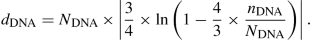  (3.1)

  • The formula is intended to correct for the occurrences of multiple nucleotide substitutions at the same site (nucleotide position). A correction would be needed since the number of nucleotide differences at a site cannot be more than 1.

  • Note that the formula only works well when is small. For a very large numeric value of , it can happen that or . In those cases, resetting to works well with the method of Sect. 3.1.2.1, for that creates ties that tend to avoid applying its Step 5 of Sect. 3.1.2.1 beyond the scope recommended by Hall [53, pp. 80–81], following Nei and Kumar [92]. For real data, a large may indicate a lack of homology between the sequences or, as Hall [53, pp. 60–62] discusses, that they are poorly aligned with each other.

  • With that distance matrix, create the DNA-based corrected tree by following the steps of Sect. 3.1.2.1.

  • The Jukes–Cantor correction applies not only to constant-rate models but also to those allowing the rate of substitution to vary over time (Sect. 3.5.3).

3.2 Relations of Different Types of Trees

The main ideas of Substituter are organized in Fig. 3.5 in terms of these six trees:

Fig. 3.5

Five trees from one expected tree

• (1) Expected tree (Fig. 3.1)

• (2) Realized tree (Sect. 3.1.1)

• (3) Uncorrected protein-based tree (Sect. 3.1.2.1)

• (4) Uncorrected DNA-based tree (Sect. 3.1.2.1)

• (5) Corrected protein-based tree (Sect. 3.1.2.2)

• (6) Corrected DNA-based tree (Sect. 3.1.2.3)

An alignment is a set of sequences edited to facilitate comparisons between their homologous building blocks. Each expected tree corresponds to one alignment: for each expected tree, all of the tip sequences together constitute one alignment.

Each alignment may be used with the steps of Sects. 3.1.2.1, 3.1.2.2, and 3.1.2.3 to estimate trees. Section 3.3 explains how to automate estimating trees from an alignment saved as a computer file. Uncertainty due to potential alignment errors is described in Sect. 3.4.1.

3.3 Software for Tree Estimation

These steps explain how to use MEGA X [74, 108] to estimate phylogenetic trees:

• (1) Install MEGA X after downloading it from https://www.megasoftware.net.

• (2) On your computer, find and double-click the “Crab_rRNA.meg” alignment file mentioned in the MEGAX-Help tutorial page at https://bit.ly/3lGqfgh (“Building Trees From Sequence Data”).

• (3) Examine the alignment to see which sequences are being compared and how they are positioned relative to each other.

• (4) Follow the tutorial steps to construct a Neighbor-Joining (NJ) tree (Example 4.1 of the tutorial), for “Model/Method” selecting “p-distance.” (“No. of differences” is what you used when you played Substituter, but if you divide it by the number of sites, you get the “p-distance.”)

• (5) Follow the same steps to construct a UPGMA tree instead of a NJ tree by clicking “PHYLOGENY” and then “Construct/Test UPGMA Tree…” instead of “Construct/Test Neighbor-Joining Tree…” (The UPGMA method is more like what you used when you played Substituter.)

• (6) Select each window with a tree and click “View,” “Show/Hide,” and “Branch Lengths.” That shows the numbers of differences.

• (7) Follow the above steps except this time for “Model/Method” selecting “Jukes–Cantor model” instead of “p-distance.” (That is the distance-correction method you used when you played Substituter when dividing by the number of sites.) This time, showing the branch lengths displays the corrected distances.

By following those steps, you have created four of the trees mentioned in Fig. 3.6. To complete Exercise 3, you will also do so using the “mtCDNA.meg” and “Drosophila_Adh.meg” alignment files that came with MEGA X instead of the “Crab_rRNA.meg” alignment file. (In Substituter, your team generated a DNA alignment of three sequences for each of the expected trees (A, B, C, and D), for a total of four three-sequence alignments.)

Fig. 3.6

2 distance methods × 3 substitution models = 6 estimates of trees. The first four tree estimates are generated by following the steps of Sect. 3.3. For more information on substitution models, see Sect. 3.5

3.4 Sources of Uncertainty in Tree Estimates

As seen in Chap. 1, each reconstructed tree is only an estimate based on many assumptions that are incorrect to varying and usually unknown degrees. Each source of uncertainty contributes to uncertainty about the estimated tree. The following sources of uncertainty have received the most attention.

3.4.1 Uncertainty About Common Ancestry

Phylogenetic tree estimation assumes the present-day sequences included in an alignment (Sect. 3.2) are homologous in the sense of having evolved from a common ancestor (Sect. 1.2.1). On the one hand, a high degree of sequence similarity, perhaps quantified by an extremely low E value in the BLAST software, suggests homology [53, chapter 3]. On the other hand, homology cannot be inferred from similarity alone, as clearly explained by Lesk [82, pp. 159–160].

Inadvertently including nonhomologous sequences in an alignment introduces errors in tree estimates that even affect the probabilities associated with the sequences in the alignment that are in fact homologous. Too much error of that type would mean the tree could not be interpreted in terms of evolutionary relationships (Sect. 1.2.1).

Xia [132, chapter 2] observes that many published phylogenetic trees suffer biases due to poor sequence alignment. Xia [132, chapter 2] further laments that journal editors tend to favor the publication of trees so large that peer reviewers cannot check all of the alignments. Even when care is taken to align the sequences as well as possible, different alignment algorithms make different assumptions, requiring researchers to try different algorithms on the same sequences in order to assess how much influence the algorithm has on the conclusions [132, chapter 2].

Any resulting uncertainty about the alignment increases the uncertainty about the estimated trees. That uncertainty is captured to some extent in Substituter since the sequences simulated from “Tree A” of Fig. 3.1 are incorrectly considered homologous by the team working in estimation mode (Sect. 3.1.2).

3.4.2 Uncertainty About the Topology

Uncertainty in the topology of a tree is often indicated by collapsing a bifurcation (e.g., Fig. 3.4) into a polytomy (e.g., Fig. 3.3). For example, that is what Step 4 of Sect. 3.1.2.1 does. Some of this uncertainty may be represented by the bootstrap measure of certainty to be covered in Sect. 4.1. It was not represented in Step 2 of Sect. 5.3 since the topology of the expected tree was used.

3.4.3 Uncertainty About the Branch Lengths

Even if the topology of part of a tree is correct, the branch lengths associated with that part cannot be known very precisely. Uncertainty about branch lengths leads to uncertainty about speciation rates and other biological quantities calculated from estimates of branch lengths. For example, uncertainty in the rate of evolution, even when neglecting other sources of uncertainty, would lead to errors in a measure of biodiversity from 10% to 38%, which is large enough to affect practical decisions about conservation [103].

Some of the uncertainty about branch lengths can be represented with confidence intervals, as will be seen in Sect. 4.2.2. It was not represented in Step 2 of Sect. 5.3 since the branch lengths of the expected tree were used. However, even confidence intervals corrected by the method of 4.1 fail to quantify all uncertainty since they depend on assumptions made by the substitution model.

3.4.4 Uncertainty About the Substitution Model

Every method of estimating a phylogenetic tree needs a mathematical model of substitutions. A simple model is the Poisson model that underlies the rules of Substituter (Sect. 3.1.1.1). Examples of more realistic models are mentioned in Sect. 3.5.

More realism in a model can improve estimation unless the model is too realistic in the sense of being too complex compared to the amount of data available. That is because accurately estimating numbers of substitutions even though many of them are hidden by other substitutions (Sect. 1.1) requires a substitution model that is neither too simple nor too complex. The model of substitution must be complex enough to capture the main features of molecular evolution and yet not overly complex, lest it fit the data so well that it does not generalize to past events [27].

Statistical tests are available to check the agreement of models with data. However, if all of the available substitution models fail the statistical tests, a researcher may react by discarding the sequences that lead to those test outcomes. Unfortunately, deleting those sequences may bias the results [27].

A portion of the uncertainty about the model can be assessed by trying different substitution models and noting how they affect the estimates [26, p. 448]. A more algorithmic solution is to compute the confidence interval of a branch length for each model and then to report the lowest and highest limits [cf. 19]. That approach is discussed further in Sect. 4.2.1. It may also be used to quantify the uncertainty about the tree estimation method.

A mathematical way to represent uncertainty about the model appears in Sect. A.3 of Appendix A.

3.4.5 Uncertainty About the Tree Estimation Method

Various methods of phylogenetic tree estimation include UPGMA, neighbor joining, and minimum evolution (Sect. 3.1.2.1). Some of this uncertainty can be assessed by trying different tree estimation methods and noting how they affect the topologies and branch lengths.

3.4.6 Uncertainty About the Statistical Method and Prior Probabilities

Uncertainty about the statistical method and about prior probabilities (Sect. 1.2.3) tends to have large impacts on the uncertainty about the branch lengths and topologies of trees. These sources of uncertainty are described in Sects. 4.2.1 and 5.5.1.

Here, it is enough to note that while Bayesian posterior probabilities of clades have been reported to be misleadingly high [134], the bootstrap proportion (Sect. 4.1), often used with maximum likelihood methods, tends to be on the conservative side [19, 56, 136].

3.5 Excursus: Models of Nucleotide Substitution

The focus of this optional section is on nucleotide substitutions, but the statistical methods apply to amino acid substitutions with little modification [43, §13.1]. In practice, uncertainty about which substitution model to use propagates to uncertainty in the results (see Sect. 3.4.4).

3.5.1 Background Terminology

Recall from Sect. 1.1 that a substitution is a change of which amino acid or nucleotide at a certain protein or DNA site is predominant in a given population. A transition is the substitution of one purine (adenine or guanine) for the other purine or of one pyrimidine (cytosine or thymine) for the other, whereas a transversion is the substitution of a purine for a pyrimidine or vice versa. ewens2001statistical ]

3.5.2 Discrete-Time Models [43, §13.2]

These models treat time as discrete in the sense of being represented in integer numbers of time units:

• Discrete-time Jukes–Cantor model. This model has only one parameter, the nucleotide substitution rate. The simple symmetric PAM model is the amino acid version of the Jukes–Cantor model. Other PAM models of amino acid substitutions are more realistic.

• Kimura models. The original Kimura model has two parameters, the rate of transitions and the rate of transversions, the latter of which is lower. There is also a three-parameter Kimura model. Another three-parameter generalization has different rates for purine-to-pyrimidine and pyrimidine-to-purine substitutions. Generalizations with more than three parameters have also been suggested.

• Felsenstein model. Felsenstein proposed a model that generalizes both the Jukes–Cantor model and a Markov chain. The Felsenstein model is reversible in the sense that it has the same stationary distribution backward in time as it does forward in time [43, §10.2.4]. Reversibility is important when comparing two sequences with an unknown common ancestor since in that case the direction of time cannot be determined for all substitutions. A reversible generalization of the Felsenstein model has been proposed.

• HKY model. The HKY model generalizes both the two-parameter Kimura model and the Felsenstein model.

• Rate-varying models. More complex models do not assume that all sites on a sequence evolve at the same rate. A popular model of this type assumes a gamma distribution of rates.

ewens2001statistical ]

3.5.3 Continuous-Time Models [43, §13.3]

These models drop the assumption of discrete time:

• Continuous-time Jukes–Cantor model. Numbers of substitutions in the continuous-time Jukes–Cantor model [64] follow the homogeneous (constant-rate) Poisson distribution. This model corrects for multiple and back substitutions (see Sect. 1.1) in the estimation of the number of substitutions that took place since divergence from a common ancestor, as follows. Given the proportion of sites that differ between two sequences, one can use Eq. (3.1) to estimate the number of substitutions.

  • Bickel and West [20] used a doubly stochastic Poisson process to demonstrate that Eq. (3.1) also applies to the case of a rate of evolution that fluctuates in time, assuming that the mean rate of substitution is both stationary and the same for transitions and transversions.

  • Nei and Kumar [92, p. 37] derived equation (3.1) from the discrete-time Jukes–Cantor model mentioned in Sect. 3.5.2.

• Other continuous-time models. There are continuous-time versions of the discrete-time models described in Sect. 3.5.2.

3.5.4 Further Reading

Section 3.5 closely follows Ewens and Grant [43, chapter 13], which may be consulted for details and additional references to the primary literature. That book is recommended in Sect. 7.1.2.

3.6 Exercises

• (1) After identifying the members of two competing teams, work with your team to defeat the opposing team.

  • (a) After following the rules of Sect. 3.1.1, your team will work in simulation mode to generate the sequence data the opposing team needs for Exercise 1b.

    • It is strongly recommended that all sequences and trees generated in the following steps are clearly organized in a cloud service such as Google Docs or another location that is easily accessible by all members of your team. Depending on what technology you use for that, clear organization may involve detailed file or note names, folders or directories, and tags or labels.

      • That will help not only with the current level of Substituter but also with the next level. The rules for the next level are given in Sect. 5.2.

      • This recommendation also applies to scanned copies of any drawings made on paper.

  • (b) Follow the rules of Sect. 3.1.2 in estimation mode for an alignment provided by the opposing team. Your team will then be ready for these exercises:

    • (i) Organize the four estimated trees you generated as follows. Draw two lines to divide a blank sheet of real or virtual paper into four quadrants, like those of the right-hand side of Fig. 3.5:

      • (A) In the top-left quadrant, draw your uncorrected protein-sequence tree. Fill in its uncorrected branch lengths and tip protein sequences. Next to the tree, put its uncorrected distance matrix.

      • (B) In the bottom-left quadrant, draw your corrected protein-sequence tree. Fill in its corrected branch lengths and tip protein sequences. Next to the tree, put its corrected distance matrix.

      • (C) In the top-right quadrant, draw your uncorrected DNA-sequence tree. Fill in its uncorrected branch lengths and tip DNA sequences. Next to the tree, put its uncorrected distance matrix.

      • (D) In the bottom-right quadrant, draw your corrected DNA-sequence tree. Fill in its corrected branch lengths and tip DNA sequences. Next to the tree, put its corrected distance matrix.

    • (ii) Are the topologies of your two protein-based trees (one uncorrected and the other corrected) the same or different?

    • (iii) Are the topologies of your two DNA-based trees (one uncorrected and the other corrected) the same or different?

    • (iv) Are the topologies of your two corrected trees (one protein-based and the other DNA-based) the same or different?

    • (v) Which of the four expected trees of Fig. 3.1 do you think the opposing team used to generate the sequences it gave you? Why?

    • (vi) Organize the endgame as follows. Draw two lines to divide a blank sheet of real or virtual paper into four quadrants.

      • (A) In the top-left quadrant, copy your DNA-based corrected tree (with its branch lengths and tip DNA sequences) from Step 1(b)iD.

      • (B) In the bottom-left quadrant, draw what you guess is the expected tree, knowing it is one of the trees displayed in Fig. 3.1.

      • (C) Tell the opposing team which expected tree you just guessed in Exercise 1(b)viB. After that, ask the opponent which expected tree is correct, and then draw it in the top-right quadrant.

      • (D) In the bottom-right quadrant, draw the realized tree provided by the opponent (with its branch lengths and with the DNA sequences of its tips).

  • (c) Who won? Scoring for the DNA-based corrected trees:

    • (i) Gain 10,000 points for each correctly guessed expected tree.

    • (ii) Section 3.2 and Fig. 3.5 explain what the “realized tree” is. Does your DNA-based corrected tree have the same topology as the realized tree?

      • (A) If so, then lose 1000 points for every substitution that the branch lengths of your expected DNA-based tree differ from those of the realized tree.

      • (B) If not, then lose 10,000 points.

  • (d) Estimated trees versus the true tree:

    • (i) What does playing Substituter tell you about the distinction between the realized tree and an estimated tree? Again, Sect. 3.2 and Fig. 3.5 explain what the “realized tree” is.

    • (ii) Which sources of uncertainty listed in Sect. 3.4 contributed to the differences you saw in Exercise 1(c)ii between the realized tree and the estimated tree?

    • (iii) Which sources of uncertainty listed in Sect. 3.4 are in nature but not in Substituter?

  • (e) More takeaways from Substituter:

    • (i) What is the purpose of each of the six trees listed in Sect. 3.2? Hint: Fig. 3.5.

    • (ii) Which tree corresponds to the process of molecular evolution?

    • (iii) Which four trees are only estimates of that tree?

    • (iv) How does the remaining tree relate to the molecular clock hypothesis (Sect. 1.2.2)?

• (2) Real data:

  • (a) Create both the protein-based uncorrected tree and the protein-based corrected tree for the 3 sequences of Fig. 3.7.

    Fig. 3.7

    

    Number of amino acids different =  number of amino acid sites in the alignment − number of amino acids the same. Data source: Lesk [82, p. 158, Case Study 4.4]

  • (b) Are their topologies the same or different?

  • (c) What are the branch lengths?

  • (d) How close do you think your estimated trees are to what really happened in evolution? Hint: review the sources of uncertainty listed in Sect. 3.4 and your answer to Exercise 1d.

• (3) Follow the steps of Sect. 3.3 to answer these questions for each of the alignment files it mentions:

  • (a) How does applying the Jukes–Cantor correction affect the neighbor-joining tree?

    • (i) How does it affect the topology (which sequences are in the same cluster)?

    • (ii) How does it affect the branch lengths?

  • (b) How does applying the Jukes–Cantor correction affect the UPGMA tree?

    • (i) How does it affect the topology?

    • (ii) How does it affect the branch lengths?

  • (c) Considering only the trees using the Jukes–Cantor correction, compare the neighbor-joining tree to the UPGMA tree.

    • (i) Do they have the same topology?

    • (ii) How different are their branch lengths?

  • (d) This exercise illustrates some of the sources of uncertainty listed in Sect. 3.4.

    • (i) Which of those sources of uncertainty are considered?

    • (ii) Which of those sources of uncertainty are not considered?

References

Bayer, O. 2012. A Contemporary in Dissent: Johann Georg Hamann as Radical Enlightener. Grand Rapids: Wm. B. Eerdmans Publishing.
Bickel, D.R. 2022c. Propagating clade and model uncertainty to confidence intervals of divergence times and branch lengths. Molecular Phylogenetics and Evolution 167: 107357.
Bickel, D.R., and B.J. West. 1998a. Molecular evolution modeled as a fractal Poisson process in agreement with mammalian sequence comparisons. Molecular Biology and Evolution 15: 967–977.
Bromham, L. 2016. An Introduction to Molecular Evolution and Phylogenetics. Oxford: Oxford University Press.
Bromham, L. 2019. Six impossible things before breakfast: Assumptions, models, and belief in molecular dating. Trends in Ecology & Evolution 34: 474–486.
Ewens, W.J., and G.R. Grant. 2001. Statistical Methods in Bioinformatics: An Introduction. Statistics for Biology and Health. Berlin: Springer.
Hall, B. 2018a. Phylogenetic Trees Made Easy: A How-To Manual. New York: Sinauer Associates.
Hillis, D.M., and J.J. Bull. 1993. An empirical test of bootstrapping as a method for assessing confidence in phylogenetic analysis. Systematic Biology 42: 182–192.
Jukes, T.H., and C.R. Cantor. 1969. Evolution of protein molecules. Mammalian Protein Metabolism 3: 21–132.
Kumar, S., G. Stecher, M. Li, C. Knyaz, and K. Tamura. 2018. MEGA X: Molecular evolutionary genetics analysis across computing platforms. Molecular Biology and Evolution 35: 1547.
Lesk, A. 2019. Introduction to Bioinformatics. Oxford: Oxford University Press.
Nei, M., and S. Kumar. 2000. Molecular Evolution and Phylogenetics. Oxford: Oxford University Press.
Ritchie, A.M., X. Hua, M. Cardillo, K.J. Yaxley, R. Dinnage, and L. Bromham. 2021. Phylogenetic diversity metrics from molecular phylogenies: modelling expected degree of error under realistic rate variation. Diversity and Distributions 27: 164–178.
Stecher, G., K. Tamura, and S. Kumar. 2020. Molecular evolutionary genetics analysis (MEGA) for macOS. Molecular Biology and Evolution 37: 1237–1239.
Xia, X. 2020. A Mathematical Primer of Molecular Phylogenetics. New York: Chapman and Hall/CRC.
Yang, Z. 2014. Molecular Evolution: A Statistical Approach. Oxford: Oxford University Press.
Yang, Z., and T. Zhu. 2018. Bayesian selection of misspecified models is overconfident and may cause spurious posterior probabilities for phylogenetic trees. Proceedings of the National Academy of Sciences 115: 1854–1859.
Zharkikh, A., and W.H. Li. 1992. Statistical properties of bootstrap estimation of phylogenetic variability from nucleotide sequences. I. Four taxa with a molecular clock. Molecular Biology and Evolution 9: 1119–1147.
Author information
Authors and Affiliations
3.1 Electronic Supplementary Materials
Supplemental 1
ancestor uncertainty (xlsx 1021 kb)
Rights and permissions
Copyright information
© 2022 The Author(s), under exclusive license to Springer Nature Switzerland AG
About this chapter
Cite this chapter
Bickel, D. (2022). Estimating Phylogenetic Trees. In: Phylogenetic Trees and Molecular Evolution. SpringerBriefs in Systems Biology. Springer, Cham. https://doi.org/10.1007/978-3-031-11958-3_3
Download citation
DOI: https://doi.org/10.1007/978-3-031-11958-3_3
Publisher Name: Springer, Cham
Print ISBN: 978-3-031-11957-6
Online ISBN: 978-3-031-11958-3
eBook Packages: Biomedical and Life SciencesBiomedical and Life Sciences (R0)