
Abstract
This article focuses on the issue of optimising the transport process of cargo-intensive sections analyses the section capacity and outlines the most relevant ways of increasing carrying capacity and throughput today. In order to reduce capital expenditures for capacity enhancement the optimization task on revealing and determining the factors’ values influencing the carrying capacity was formed. Rational location of locomotive fleet on the sections allows to increase weight standards of goods trains on the one hand and on the other hand with useful track length less than 1050 m a reserve of locomotive capacity appears. On sections with low gradient up to ip < 8‰ the reserve should be used to increase running speed while on sections with difficult profile ip > 20‰ the reserve should be used to increase weight standards of the train. The proposed methodology made it possible to determine the optimum values of weight norms and speeds on the basis of the obtained values of running speed parameters and the division of the train traffic into three categories (light, mixed and heavy) using the optimum type of locomotive 2TE116. The results obtained prove the relevance of the study and show that the main factor that has a significant impact on carrying capacity is the locomotive performance. When determining carrying capacity the average train weight should be used rather than the weight standard set by the train schedule.
Access provided by Autonomous University of Puebla. Download conference paper PDF
Keywords
1 Introduction
The transport capacity of railway lines is determined by their carriage and throughput capacity. In the face of capacity and carrying capacity shortages on railway lines there is a need to analyse the key factors affecting capacity [1]. An assessment of the available freight carrying capacity of railroad sections with critical infrastructure elements [2] shows the need to investigate and find specific solutions for determining the capacity and freight carrying capacity and to optimise the routes [3] and the size of goods train movements as noted in the authors’ work [4,5,6].
Classification of goods trains by weight and speed (heavy, mixed and light) based on the technical characteristics and fleet parameters of different types of freight wagons] allows longer and heavier trains to be operated when allocating traction capacity of the locomotive fleet [7, 8].
Energy efficiency and train length can be crucial in determining capacity especially when limiting the length of the station line [9, 10].
It is known that capacity is directly related to three main parameters:
-
capacity, i.e. the maximum possible number of goods trains that a given line can carry per unit time in a parallel timetable [11];
-
the operational parameters of the wagon fleet the impact of in terms of wagon fleet utilisation factor,
-
the net weight of a goods train that might be realised under the given conditions on that line [12].
The value of the boundary gradient affects the weight rating of trains and the carrying capacity of the designed railway section. It determines the complexity of the longitudinal profile, travel speeds, fuel or energy consumption.
The track profile has a significant role amongst the external forces that impede the train’s movement. On average, the mechanical work inputs of locomotive traction to overcome the traffic resistance of goods trains are distributed as follows: 60% - basic resistance, 35% - track profile gradients, 5% - track curvature. On average, the mechanical work inputs of locomotive traction to overcome the traffic resistance of goods trains are distributed as follows: 60% - basic resistance, 35% - track profile gradients, 5% - track curvature.
If the speed of the trains is unchanged use to increase their weight and length, then the capacity of the section will decrease but the carrying capacity will increase allowing fewer trains to carry significantly more wagons (freight) [13].
2 Materials and Methods
-
1.
Capacity dependence on individual factors
-
1.1.
Problem statement, main factors
-
1.1.
The capacity value is determined by the formula:
Where \(N_{f} \) – capacity for freight traffic, train pairs.
\(\varphi\) – the wagon fleet utilisation factor;
\(Q_{gr}^{av}\) – average train weight, t;
Qgr – the weight standard of the train set in the timetable, t;
\(kn\) – is the coefficient of monthly traffic irregularity.
Z – the coefficient of the weight rate utilisation set in the timetable,
It is known that the carrying capacity of a railway line (section) is determined by the carrying capacity of its technical equipment elements: runs, track development of intermediate and technical stations, power supply system, locomotive facilities, signalling and communication system, etc.
Consider the line capacity determined by the bounding line. The throughput with a parallel schedule then depends on the travel speed (\(V_{r}\)), the station intervals (τs) and the acceleration and deceleration times (\(t_{as}\)). In general terms, the nature of this dependence is expressed by the following formula:
Where \(L_{lim}\) is the length of the boundary line, km.
The wagon fleet utilisation factor \( \varphi\) is expressed in terms of average weight or wagon capacity utilisation factor (Klp):
Where \(q_{n}\) – net wagon load, tonnes;
\(q_{gr}\) – the average gross wagon weight, tonnes;
\(K_{lp} \) – the load capacity utilisation factor of the wagon,
\(q_{lp }\) - wagon load capacity, tonnes.
\({\text{k}}_{{\text{c}}}\) - the wagon tare factor,
Formulas (1)–(3) show that the reserves for improving the capacity of railway lines are increasing the running speed of the goods train, reducing the station intervals, improving the performance of the rolling stock and increasing the average weight of the goods train.
For the purpose of this study let us consider the factors that determine the average weight of a goods train. The main ones are locomotive pulling power, track profile and useful length of the receiving track. In addition, the freight flow in each direction is significantly influenced by the completeness of the goods trains and therefore the static load of the wagons and the structure of the wagon fleet (availability of four- and eight-axle wagons). The static load of wagons is increased by densified loading and rational allocation of empty wagons for loading of certain types of cargo [14].
Rational deployment of the locomotive fleet on the railways also allows for higher weight standards for goods trains [15]. It is important to allocate the most powerful locomotives for sections with difficult profile conditions and for lines where the main flows are heavy loads. Low-power locomotives should be used on the easiest profile conditions. The train’s weight has two limitations:
-
1)
in terms of locomotive traction force
$$ Q_{gr} \le { }\frac{{F_{ap} - P\left( {W^{\prime}_{o} + i_{\rm{p}} } \right)}}{{{ }W_{o}^{\prime \prime } + i_{p} { }}} $$(7)
Where \(F_{ap}\) is tangential traction force of the locomotive, kN;
P – locomotive weight, tonnes;
\(W^{\prime}_{o}\), \({ }W_{o}^{\prime \prime }\) – is the basic specific resistance of the locomotive and wagons respectively at design speed, N/kN;
\(i_{p}\) – design elevation, ‰.
-
2)
along the station track length:
$$ Q_{gr} \le \left( {L_{s} - L_{l} } \right)q $$(8)
Where \(L_{s}\) – usable track length, m;
\(L_{l}\) – locomotive length including distance to stop accuracy within usable track length, m;
\(q_{ }\) – design load from the static distribution series, t/m2.
The weight standards set in terms of locomotive pulling power ensure better use of the locomotive. The weight standards set by track length at the highest line load ensure the smallest traffic sizes. When heavy trains are used the issue arises of the underutilisation of station track length and the unjustified increase in traffic size. When light trains are used there is excess locomotive capacity which can partially be used to increase running speeds.
This raises the problem of selecting the optimum train weights and traction support for the transport process.
Let’s show one possible solution to this problem.
Taking into account (1)–(3) the carrying capacity as a function of train weight and throughput as well as the operational parameters of the wagon fleet can be expressed as follows:
-
1)
When limiting train weight by locomotive pulling power using formula (4)
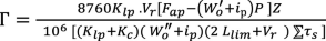 (9)
(9)

-
2)
When limiting train weight by track length using (5)
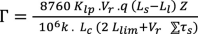 (10)
(10)

Based on the analysis of the dependence of capacity on individual factors the following may be noted. The estimated train weight is significantly influenced by the degree to which the lifting power of the wagons is utilised. The lower the steering gradient and the higher the speed of goods trains on this gradient the greater the effect of wagon weights on the calculated train weight.
The saturation of the wagon fleet with heavy multi-axle wagons with high loads can significantly increase capacity. Currently, Russian Railways is introducing new technology for the use of cassette-type tapered axlebox bearings making it possible to significantly increase the weight and speed of goods trains for the same length of station tracks.
Where the effective length of the station tracks is less than 1,050 m this raises the issue of locomotive capacity underutilisation. Therefore, on sections with low gradients up to ip < 8‰ the underutilised power can be allocated to increase the travelling speed. On sections with large rises of ip > 20‰ it can be directed towards ensuring weight standards.
It follows from the above that the weight of a goods train on railway sections with low gradients is determined not by the type of locomotive but by the length of station tracks and the calculated load depending on the freight turnover structure and the wagon fleet [16,17,18]. As a result, the impact of the locomotive on the line capacity becomes significant on the sections with high gradients when on the other sections (with light gradients) the level of train speed of a given weight realized with a given locomotive becomes decisive [19, 20].
When locomotive pulling power is limited it is possible to increase the weight of a goods train by
-
1)
increasing the tangential pulling power of the Far locomotive (new pulling, nudging, connection of additional sections, introduction of more powerful locomotives) while increasing the tangential pulling power of the locomotive; \(Q_{gr} \)
-
2)
reduction of the wagon’s tare utilisation factor. In this case it is possible to increase the net weight of the train.
3 Results Analysis
As already shown in (6) and (7) capacity is directly related to gross train weight and running speed of goods trains:
The work
Characterises the performance of a locomotive. The D value must be maximised in order to obtain the highest capacity. This requires either accurate traction calculations for different gradations of train weight on the bounding line or an analytical determination of the relationship between running speed and gross train weight:
This dependency was first identified by Professor N.A. Vorobiev
Where a and b are parameters that take into account the running speed of goods trains.
One of the authors of this article carried out traction calculations using a 2TE116 diesel locomotive where parameters a и b depending on profile types including for mountainous terrain were derived (Table 1).
Using the data in the table the dependence of locomotive performance D o on the obtained dependence shows that with some Qcr the value of D takes the maximum value. A further increase in the average train weight leads to a decrease in locomotive performance associated with a decrease in running speed [21, 22].
Thus, it is possible to increase the capacity of a line by increasing the average train weight to Qcr with some reduction in running speed. Increasing the average train weight above the value \(Q_{gr}\) is not advisable as it leads to a reduction in capacity Fig. 1

Locomotive performance as a function of average train weight

Train weight vs steepness of design gradient with diesel locomotive traction
Figure 2 shows the relationship between train weight and steering gradient when operating different types of locomotives.
Determining the optimum average weight of a goods train.
To justify the average train weight standard using formulas (9) and (10) carry out the following conversions:
Let us differentiate the resulting expression:
We express a by
 :
:
Then the optimum value of the average train weight \( Q_{op}\) will be:
The resulting expression can be used to determine the optimum value for the average train compound.
Since \(Q_{gr} = l_{c}\)\(. q_{ } , \) a m = \( \frac{{l_{c } }}{14}\) = \( \frac{{Q_{gr} }}{{14 . q_{ } }}\) we have:
Where \(m_{c}\) is the train’s train size limited by the length of the station’s receiving and departing tracks, m; \(l_{c} -\) train length, meters.
4 Summary
An important element in organising the operational work of railways is the weight and length of goods trains affecting the throughput and carrying capacity of sections. One of the main solutions for increasing the carrying capacity of freight sections and routes is to optimise the weight standards and running speeds of goods trains and to efficiently distribute the traction capacity of the locomotive fleet.
The above methodology provides a consistent solution for setting the average train weight, the length of the receiving track and the average train composition.
5 Conclusion
-
1.
The main factor that has a significant impact on the capacity of a rail line is the locomotive performance depending in turn on the average weight of the train and the running speed.
-
2.
A certain average train weight corresponds to the maximum carrying capacity deviating from this value either to the lower or to the higher side will result in a negative result - a reduction in carrying capacity.
-
3.
When determining capacity the average train weight should be used rather than the weight standard set in the train timetable.
-
4.
With constant station track lengths the difference between the average train weight and the graphical weight standard shows that there are reserves for increasing the train weight.
References
Fenling, F., Dan, L.: Prediction of railway cargo carrying capacity in China based on system dynamics. Procedia Eng. 29, 597–602 (2012). https://doi.org/10.1016/j.proeng.2012.01.010
Pascariu, B., Coviello, N., D’Ariano, A.: Railway freight node capacity evaluation: a timetable-saturation approach and its application to the Novara freight terminal. Transp. Res. Procedia 52, 155–162 (2021). https://doi.org/10.1016/j.trpro.2021.01.017
Zhengwen, L., Haiying, L., Jianrui, M., et al.: Railway capacity estimation considering vehicle circulation: Integrated timetable and vehicles scheduling on hybrid time-space networks. Transp. Res. Part C Emerg. Technol. 124, 102961 (2021). https://doi.org/10.1016/j.trc.2020.102961
Mussone, L., Calvo, R.W.: An analytical approach to calculate the capacity of a railway system. Eur. J. Oper. Res. 228(1), 11–23 (2013). https://doi.org/10.1016/j.ejor.2012.12.027
Khaled, A.A., Mingzhou, J., Clarke, D.B., Mohammad, A.: Hoque, train design and routing optimization for evaluating criticality of freight railroad infrastructures. Transp. Res. Part B Methodol. 71, 71–84 (2015). https://doi.org/10.1016/j.trb.2014.10.002
Dolgopolov, P., Konstantinov, D., Rybalchenko, L., et al.: Optimization of train routes based on neuro-fuzzy modeling and genetic algorithms. Procedia Comput. Sci. 149, 11–18 (2019). https://doi.org/10.1016/j.procs.2019.01.101
Schwerdfeger, S., Otto, A., Boysen, N.: Rail platooning: Scheduling trains along a rail corridor with rapid-shunting facilities. Eur. J. Oper. Res. (2021). https://doi.org/10.1016/j.ejor.2021.02.019
Siroky, J., Siroka, P., Vojtek, M., et al.: Establishing line throughput with regard to the operation of longer trains. Transp. Res. Procedia 53, 80–90 (2021). https://doi.org/10.1016/j.trpro.2021.02.011
Toletti, A., De Martinis, V., Weidmann, U.: What about train length and energy efficiency of freight trains in rescheduling models. Transp. Res. Procedia 10, 584–594 (2015). https://doi.org/10.1016/j.trpro.2015.09.012
Domanov, K., Nekhaev, V., Cheremisin, V.: Optimization of operating modes of a train by the haul distance. Transp. Res. Procedia 54, 842–853 (2021). https://doi.org/10.1016/j.trpro.2021.02.142
Ljubaj, I., Mikulčić, M., Mlinarić, T.J.: Possibility of increasing the railway capacity of the R106 regional line by using a simulation tool. Transp. Res. Procedia 44, 137–144 (2020). https://doi.org/10.1016/j.trpro.2020.02.020
Abdullaev, Z.Y.: Features of determining the capacity of two-track sections (Features of determining the capacity of two-track sections). Proc. Petersburg State Transp. Univ. 16(3), 361–371 (2019). https://doi.org/10.20295/1815-588X-2019-3-361-371
Jamili, A.: Computation of practical capacity in single-track railway lines based on computing the minimum buffer times. J. Rail Transp. Plan. Manag. 8(2), 91–102 (2018). https://doi.org/10.1016/j.jrtpm.2018.03.002
Nikiforova, G.I.: Construction of a descriptive model of the logistics chain for the delivery of goods in the interaction of rail and sea transport. Proc. Petersburg State Transp. Univ. 17(4), 545–551 (2020). https://doi.org/10.1016/S1570-6672(11)60217-1
Rybin, P.K., Gorin, R.V.: Decision support model for the effective control of train admission to port stations. Bull. Res. Results (4), 69–79 (2019). https://doi.org/10.20295/2223-9987-2019-4-69-79
Liu, Z., Zhou, X., Fang, Q.: Data mining on index of static load of freight cars. J. Transp. Syst. Eng. Inf. Technol. 12(4), 128–134 (2012). https://doi.org/10.1016/S1570-6672(11.60217-1
Nikiforova, G.I.: Research on the operation of the car fleet of operator companies. Proc. Petersburg Transp. Univ. 17(3), 282–287 (2020). https://doi.org/10.20295/1815-588X-2020-3-282-287
Kovalev, K.E., Kizlyak, O.P., Galkina, J.E.: Automation of management functions of operational personnel of railway stations. In: 2019 International Multi-Conference on Industrial Engineering and Modern Technologies, FarEastCon: 8933836 (2019). https://doi.org/10.1109/FarEastCon.2019.8933836
Milenković, M.S., Bojović, N.J., Švadlenka, L., et al.: A stochastic model predictive control to heterogeneous rail freight car fleet sizing problem. Transp. Res. Part E Logistics Transp. Rev. 82, 162–198 (2015). https://doi.org/10.1016/j.tre.2015.07.009
Armstrong, J., Preston, J.: Capacity utilization and performance at railway stations. J. Rail Transp. Plan. Manag. 7(3), 187–205 (2017). https://doi.org/10.1016/j.jrtpm.2017.08.003
Abdullaev, Z.Y., Groshev, G.M., Grachev, A.A., et al.: The choice of railway train load and length rate. Bull. Sci. Res. Res. 2019(3), 25–37 (2019). https://doi.org/10.20295/2223-9987-2019-3-25-37
Weik, N., Warg, J., Johansson, I., et al.: Extending UIC 406-based capacity analysis – new approaches for railway nodes and network effects. J. Rail Transp. Plan. Manag. 15, 100199 (2020). https://doi.org/10.1016/j.jrtpm.2020.100199
Author information
Authors and Affiliations
Editor information
Editors and Affiliations
Rights and permissions
Copyright information
© 2022 The Author(s), under exclusive license to Springer Nature Switzerland AG
About this paper

Cite this paper
Al-Shumari, A. (2022). Weight and Speed Optimization for Goods Trains on Cargo-Intensive Railway Sections. In: Manakov, A., Edigarian, A. (eds) International Scientific Siberian Transport Forum TransSiberia - 2021. TransSiberia 2021. Lecture Notes in Networks and Systems, vol 402. Springer, Cham. https://doi.org/10.1007/978-3-030-96380-4_24
Download citation
DOI: https://doi.org/10.1007/978-3-030-96380-4_24
Published:
Publisher Name: Springer, Cham
Print ISBN: 978-3-030-96379-8
Online ISBN: 978-3-030-96380-4
eBook Packages: EngineeringEngineering (R0)