
Abstract
Monitoring of Land use and Land cover (LULC) changes is a highly encumbering task for humans. Therefore, machine learning based classification systems can help to deal with this challenge. In this context, this study evaluates and compares the performance of two Single Learning (SL) techniques and one Ensemble Learning (EL) technique. All the empirical evaluations were over the open source LULC dataset proposed by the German Center for Artificial Intelligence (EuroSAT), and used the performance criteria -accuracy, precision, recall, F1 score and change in accuracy for the EL classifiers-. We firstly evaluate the performance of SL techniques: Building and optimizing a Convolutional Neural Network architecture, implementing Transfer learning, and training Machine learning algorithms on visual features extracted by Deep Feature Extractors. Second, we assess EL techniques and compare them with SL classifiers. Finally, we compare the capability of EL and hyperparameter tuning to improve the performance of the Deep Learning models we built. These experiments showed that Transfer learning is the SL technique that achieves the highest accuracy and that EL can indeed outperform the SL classifiers.
Access provided by Autonomous University of Puebla. Download conference paper PDF
Keywords
- Land use
- Land cover
- Machine learning
- Deep learning
- Deep feature extraction
- Ensemble learning
- Hyperparameter optimization
1 Introduction
Land use and Land cover (LULC) classification refers to the arrangement into groups of the “human activities on and in relation to the land” and the “biophysical cover of the Earth’s surface” [12, 16, 23]. LULC classification has several applications such as spanning forestry, agriculture, urban planning, and water-resources management [22]. And thanks to the availability of images of the Earth’s surface (remote sensing) and to image processing techniques, researchers can construct their own LULC dataset depending on the LULC classification problem they are dealing with. For instance, the community has already produced several open source LULC datasets (e.g. Merced Land Use [29], UC HistAerial [21], EuroSAT [9]).
To solve LULC classification problems, the literature suggests different approaches, and Convolutional Neural Networks (ConvNets) are still the most popular one [5], as they integrate the tedious feature extraction from the input images [19]. Besides, ConvNets have recently achieved major successes in many Computer Vision (CV) applications [15]. However, building ConvNets is challenging as it requires setting the values of several hyperparameters, such as the learning rate, the number of hidden layers and the batch size [17]. This drawback has motivated the use of another approach, that is Transfer learning [1, 21]. It consists of using ConvNets that were trained on an image-related task, and adapting the knowledge they had acquired to the new problem [11]. This approach reduces the time required to design and develop the models since it provides a ready to use ConvNet architecture. Nonetheless, it still leaves a set of hyperparameters to be fine-tuned by the user. Hence, the third approach we found in the previous works: Deep Feature extraction. It tries first to extract the visual features from images, and then feed them to a Machine Learning (ML) classification technique [2]. This approach achieves relatively good performance with little fine tuning. But it does not generally outperform the previously mentioned approaches [3].
The use of ML in LULC classification problems has lately proved very promising [25]. However, we noticed some limitations in the previous works, namely few pretrained models are employed and the performance of the resulting classifiers depend highly on the context. Given the cost of building new architectures, most previous works tend to use Transfer learning instead. Nevertheless, the number of Deep Learning (DL) pretrained architectures they use is still limited [1, 26]. Additionally, an important limitation when using ML/DL techniques is that different techniques give different performances depending on the context. In fact, there is no general best/worst technique in all contexts. Thus, we propose the use of Ensemble Learning (EL) techniques to remedy this limitation. The use of EL to address LULC problems is not thoroughly studied in the literature as most works focus on implementing and optimizing Transfer learning single models, and those who did employ EL techniques, have only combined ML models and did not investigate the use of DL models as members [8, 13].
This study intends to overcome the aforementioned limitations by means of: 1) thoroughly implementing single DL/ML techniques with hyperparameters optimization to find the best single model; and 2) proposing an EL approach to aggregate the performance of the best single DL/ML models.
Indeed, we firstly evaluate the three state of the art ML techniques. Specifically: we build and optimize a ConvNet architecture referred to us LULC-Net, we use several pretrained ConvNet architectures and fine tune their hyperparameters and finally we use the ConvNet part of two of these pretrained models as Feature extractors, and train ML algorithms on the resulting features. Secondly, we build different EL models: Machine Learning Ensembles (MLEnsembles), Deep Ensembles (DLEnsembles) and Hybrid Ensembles (HybridEnsembles) to solve the LULC classification problem. MLEnsembles are ensembles where the members are the ML classifiers we developed thanks to the third state of art approach (i.e. Deep Feature extraction) (see Fig. 1). DLEnsembles on the other hand are composed of DL classifiers (i.e. Transfer learning). Finally, HybridEnsembles are ensembles combining all the classifiers we built (i.e. ML and DL). Further, we study their results and investigate the use of EL as an alternative to hyperparameter tuning when it comes to improving the performance of well-performing models.
The main research contributions this paper are:
-
Evaluating three state of art single ML/DL techniques and approaches in LULC classification problems using hyperparameter optimization (i.e. new ConvNet architecture, End to End Transfer learning and Deep Feature extraction).
-
Proposing and assessing the use of different EL combinations for LULC classification.
-
Investigating the use of EL to further improve the performance of single DL models compared with hyperparameter optimization.
Thus, this study discusses the following research questions:
-
RQ1: Which one of the SL techniques (i.e. ConvNet, Transfer learning and Deep Feature extraction) performs the best on the EuroSAT dataset?
-
RQ2: Does any of the proposed EL combinations (i.e. MLEnsembles, DLEnsembles and HybridEnsembles) outperform the best SL models?
-
RQ3: Is EL a better alternative to hyperparameter tuning when it comes to increasing the accuracy of a well performing DL model?
The rest of this paper is organized as follows: Sect. 2 presents the dataset, optimization technique and evaluation metrics we chose to use in this empirical study, and discusses the hyperparameter tuning of the different models we built. Then, the performances of the SL and EL classifiers are presented and compared in Sect. 3. Section 4 provides a summary of the findings of this study and summarizes ongoing works.
2 Materials and Methods
2.1 Materials
This section presents the materials we used in this work, the experimental design and its implementation.
Dataset Description.
As part of a research project that aimed at proposing a novel dataset and DL benchmark for LULC classification, the German Center for Artificial Intelligence (DFKI)Footnote 1 constructed and made open source a new LULC dataset: EuroSAT [9]. It is composed of 27000 64 by 64-pixel images: 2000 to 3000 images per class. The team chose 10 classes of LULC that were frequent and visible in the Sentinel-2A images: Industrial Buildings, Residential Buildings, Sea and Lake, Herbaceous Vegetation, Annual Crop, Permanent Crop, River, Highway, Pasture, Forest.
Hyperparameter Optimization.
To fine tune the hyperparameters of our classifiers, we set accuracy to be the objective function and Random Search (RS) as the optimization algorithm. RS lets the hyperparameters be chosen at random within a range of values and decides the best configuration that maximizes the objective function (i.e. accuracy) [4]. It is computationally cheap, and outperforms Grid Search when some hyperparameters are far more important than others [4]. We implemented this phase using Keras Tuner [18]; a Keras hyperparameter optimization library.
Metrics.
In order to evaluate the performance of our classifiers, and since EuroSAT is a balanced dataset, this study uses the following benchmark metrics: Accuracy, Precision, Recall, and F1 score. These popular criteria are defined by Eqs. 1–4.
where TP, FP, TN and FN stand for True Positive. False Positive, True Negative and False Negative respectively. To evaluate the improvement of EL classifiers over the best single classifier, we use another metric as well, and that is Change In Accuracy. This metric compares the Accuracy of the Ensemble (AoE) to that of the Best Single Classifier (AoBSC) in the ensemble. Equation 5 defines AoBSC.
where AoBaseLearneri is Accuracy of the ith Base Learner, and N is Number of Base Learners used.
Lastly, Eq. 6 defines the Change In Accuracy metric.
where AoE(e) is Accuracy of the ensemble e, and AoBSC(e) is Accuracy of the Best Single Classifier in the ensemble e. A negative value indicates that the best single classifier outperformed the ensemble.
2.2 Experimental Design
This study focuses on providing an evaluation of the performance of diverse single ML/DL techniques in LULC classification problems and proposing a new technique based on ensemble learning as shown in Fig. 1. We used the images and labels in the EuroSAT dataset as input data, and implemented four ML approaches: build a new ConvNet architecture (LULC-Net), End to End Transfer learning, DL Feature Extraction and Ensemble Learning.
During the process of building the different classifiers, we used the following configuration: categorical cross entropy as loss function, Softmax as an activation function of the last layer and a 80–20% data split. Next, we will present the implementation details of the building process of the different classifiers.
LULC-Net:
To propose a new ConvNet architecture for LULC classification tasks, we began with a shallow ConvNet randomly configured, and while seeking to maximize the accuracy, we tuned a list of hyperparameters that according to [17] affect both the structure and the training process of ConvNets. Table 1 shows the hyperparameters we chose to tune, their respective ranges as well as the optimal values returned by the RS technique we implemented using the Keras Tuner library.
Transfer Learning.
A Transfer learning model is a combination of a DL Feature extractor (i.e. ConvNet layers) and a set of dense layers (i.e. fully connected layers). Training the Transfer learning models was a two steps process: (1) we trained the fully connected layers (initially composed of two layers, 512 and 10 neurons respectively), then fine-tuned the weights of the pretrained models. The first step trained the dense layers part of the model, and did not permit change to occur in the ConvNet part (i.e. the pretrained layers were frozen). And (2) let the learning process change the weights of the top 30% layers of the pretrained part (i.e. unfreeze the top 30% layers), and thus adapt to the new task [7] (Table 2).

Experimental design.
Deep Feature Extraction.
As it was previously pointed out, the first part of every ConvNet architecture is one that performs feature extraction [19]. Therefore, we used the convolutional part of the VGG16 and RestNet50 pretrained models to extract visual features from the images, and fed them to ML algorithms. These features are predictions of the ConvNet parts of VGG16 and RestNet50 on the EuroSAT images stored in a CSV file. And the ML models that we trained were mainly: Support Vector Machines (SVM), Random Forest (RF) and Logistic Regression (LR). Each with their default configuration implemented in the Sikit-learn library [20] (Table 3).
EL: Stacked Generalization.
We chose to develop the EL models using the stacked generalization technique, which combines learners and finds the best combination of their predictions using another model (i.e. meta learner) [27]. Figure 2 shows the implementation process we followed, we put the classifiers we built so far into three groups of base learners. The first set was composed of Deep Learners namely: VGG16, RestNet50, DenseNet201, VGG16 Places365 (VGG16-P) and VGG16HybridPlaces (VGG16-HP) (DLEnsembles) [14]. The second was made of ML models: SVM, RF, K Nearest Neighbour (KNN) and Gaussian Native Bayes (Gaussian NB) trained on the features extracted by VGG16 and RestNet50 (MLEnsembles). Finally, the last set of base learners was a combination of both approaches and sets of base learners (HybridEnsembles). The meta learners we experimented with were LR or Multilayer perceptron (MLP) and the fine tuning of this approach focused on finding the best combination of base learners and the best meta learner. By comparing the increase in accuracy introduced by EL and fine-tuning DL models we aim at investigating the ability of EL methods to improve the accuracy of well performing single models.

Ensemble learning technique.
3 Results and Final Discussion
This last section will attempt to answer the RQs of our work by presenting and discussing the findings of our work.
3.1 Performance Comparison Between ML Models
The first single classifier we built was a new ConvNet architecture: LULC-Net. Its accuracy, F1 score and training times are respectively: 94.24%, 94.36% and 7 min (12 epochs using the GPU support of Kaggle kernels). However, LULC-Net does suffer slightly from overfitting. Indeed, among the LULC classifiers we developed, the one that overfits the data the most is this newly proposed ConvNet architecture. The Transfer learning classifiers on the other hand achieved state of art performance (96% and 97% accuracy) [5, 28]. Table 4 summarizes the performance achieved by our single Transfer learning classifiers after 25 epochs of training. The DenseNet201 model achieves the best accuracy and F1 score (96.88% and 96.90% respectively). However, because of its depth [10], it takes the longest to train (30 min). On the other hand, VGG16 manages to achieve 96.81% accuracy, after just 11 min of training. Nonetheless, the performance of the VGG16 architecture decreases slightly if it was trained on the Places dataset [30] instead of ImageNet [15] (e.g. VGG16-P). One other notable finding is that InceptionV3’s performance is poor on EuroSAT compared to that of the other models we used, and this is even if InceptionV3 outperforms all of them on the ImageNet dataset [24]. Lastly, MobileNet is the pretrained model that performed the poorest on EuroSAT.
Overall the Deep Feature extraction classifiers underperformed the Transfer learning ones (see Table 5). Additionally the Deep Feature extraction model that performs the best is RestNet50 + Logistic Regression (93.86% accuracy). However, it takes RestNet50 several minutes to extract the features, which in turn elongates the classification process. Further, all metrics considered, Logistic Regression outperforms all other algorithms regardless of the Feature extractor used. In fact, it trains in fewer minutes, and it achieves the best accuracy with RestNet50’s features and second best with VGG16’s. Finally, although it takes longer to extract the features, accuracy-wise RestNet50 is a better feature extractor than VGG16. For instance, training Random Forest on RestNet50’s features improved its accuracy significantly, and that is the case for Logistic Regression as well.
In terms of accuracy and training time, the findings of the SL experiments indicate that Transfer learning performs the best, followed by LULC-Net and Deep Feature extraction classifiers. In fact, Tables 4 and 5 show that all the Transfer learning classifiers produced a better accuracy than the one ML models returned. Moreover, the experiments also demonstrate that the training time of the ML models is longer than that of the Transfer learning models: most DL models train in less than 20 min, whereas most of the ML models take more than 20 min to converge.
3.2 Performance Comparison Between EL and SL Models
The results of the experiments we conducted to answer this question show that the accuracies of the DLEnsembles and HybridEnsembles are far better than those of the MLEnsembles. In fact, the HybridEnsemble3 + LR has the worst accuracy among all DL and Hybrid ensembles (95.74%); however, its accuracy is still approximately 6% better than the accuracy of the best performing ML ensemble (i.e. MLEnsemble1 + MLP, 89.92%). Moreover, DL and Hybrid ensembles are also better at improving their Best Single Classifier’s accuracy. With the exception of the MLEnsemble4, all the ML ensembles have either slightly increased the accuracy of their Best Single Classifier (less than 0.30% increase), or decreased it. On the other hand, when they use LR as a meta learner, most of the DL and Hybrid ensembles have an accuracy that is approximately 1% better than that of their Best Single Classifier.
More insights can be drawn from Table 6. First, the best classifier this approach managed to build is a Deep EL classifier, namely: DLEnsemble1 which achieved 97.92% accuracy. Second, although DenseNet201 and VGG16 have very close accuracy values, combining DenseNet201 instead of VGG16 with VGG16-P and RestNet50 resulted in a better performing ensemble. In fact, DLEnsemble1 + LR composed of DenseNet201, VGG16-P and RestNet50 produced an accuracy of 97.92%, while DLEnsemble3 + LR where we substitute DenseNet201 with VGG16, manages to classify only 97.11% of the unseen images. Nonetheless, DLEnsemble1 takes longer to train than DLEnsemble3, and that is because DLEnsemble1 combines DenseNet201 whose time-cost is higher than VGG16’s. Similarly, ensembling the SVM classifier with KNN performed much better than MLEnsemble3. However, this high performance of ensembles where SVM is a member also comes at a high time-cost, as SVM is the model that takes the longest to train among the ML classifiers we built. Finally, the hybrid experiments show also this trade off as well: the hybrid ensembles that performed the best combined models that have the highest cost (in terms of their training time).
Finally, as a meta learner, LR outperforms MLP when the ensemble members are DL models, whereas MLP produces a better accuracy if the base learners are mainly ML. In fact, the DL ensembles + LR all returned a higher accuracy than that they produced with MLP. Similarly, the hybrid ensembles composed mostly of DL classifiers performed better with LR (accuracy-wise). On the other hand, MLP increases the accuracy of ML ensembles. With the exception of MLEnsemble3, all ML ensembles scored a higher accuracy with MLP than with LR.
3.3 Performance Comparison Between Hyperparameter Tuning and the EL Approach
Hyperparameter optimization was crucial to improving the performance of our single ML/DL models, especially the DL. Prior to fine tuning, DenseNet201 and VGG16 achieved 89% and 87% accuracy respectively. However, optimizing the same models (i.e. unfreezing their top 33% pretrained layers) increased their respective accuracies to 96.88% and 96.81%. Nonetheless, the EuroSAT benchmark model proposed by DFKI has an accuracy of 98.57% [9]. One way to increase the performance of our DL classifiers, is to extend the search space during the hyperparameter optimization. Another way is to use an EL technique and aggregate the knowledge they had previously acquired. Table 7 compares both methods as it shows the increase in accuracy of VGG16, DenseNet201 and MobileNet introduced by hyperparameter optimization and EL. The Current performance column presents the results discussed in Table 4. The third column we find the performances (accuracy and time cost) attained after further-optimizing the models; that is after unfreezing 66% of their top pretrained layers. The last column presents the performance obtained after the aggregation of the classifier in question with others in a stacked generalization ensemble. The time cost in this case is the summation of the cost of each member in the ensemble, including the meta learner.
Optimizing the hyperparameters by letting more layers adapt to the new task slightly increased the accuracy of each classifier. Actually, the model whose accuracy saw improvement the most is the MobileNet classifier, which is also the model that performed the poorest after the first fine tuning phase. More importantly, the use of EL improved all classifiers’ accuracy more than fine tuning; however, it does require more time as it trains and combines several models.
3.4 Discussion
To tackle the LULC classification from satellite images problem we used three SL approaches. The first SL approach consisted of optimizing a ConvNet architecture, and resulted in a classifier that achieves a relatively good accuracy (94%) but that overfits the data. This inability to generalize to unseen data can be due to its low expressive power, which has led to an incapacity to capture the target function. Experiments with the second approach (i.e. Transfer learning) helped us build classifiers that perform better (accuracy-wise). They also demonstrated that when it comes to LULC classification, models pretrained on the ImageNet dataset outperform the ones trained on the Places dataset; in fact, VGG16 pretrained on ImageNet achieved 96.81% accuracy and 96.33% when pretrained on Places. The third approach uses VGG16 and RestNet50 as feature extractors, stores the features they extract from EuroSAT and trains several ML algorithms on them. This last SL technique performed the poorest and some of the algorithms it uses are expensive (time-wise). The one that trains the longest is SVM, and that is due to the fact that the implementation we used is based on LIBSVM [6], which makes “the fit time scale at least quadratically with the number of samples” [20]. Overall, the SL classification technique that achieved the best results is Transfer learning. End to end classifiers outperformed the ML approach in terms of accuracy and training time. Nonetheless, this last approach and as it can use white-box ML algorithms, has the advantage of returning interpretable predictions.
To outperform the results the SL approach produced we propose the use of EL classifiers (i.e. stacked generalization) (MLEnsembles, DLEnsembles and HybridEnsembles) that combine the knowledge the SL models had gained. Overall, the findings suggest that ensembles composed of DL classifiers perform best (accuracy-wise). This should not come as a surprise since DL single learners achieve the highest accuracy among the SL models we built. Similarly, and since they performed the worst as single classifiers, ensembles of ML models also performed the poorest (accuracy-wise). All in all, the DL and ML ensembles achieved an increase in accuracy of the SL classifiers we built.
Using SL techniques, we managed to build well-performing models. In the previous Subsect. 3.3 we presented experiments that would answer our third RQ, which dealt with the viability of EL as an alternative to fine tuning when it comes to improving the performance of optimized models. However, these experiments showed once more the high accuracy and high time-cost trade-off (see Table 7). In fact, the EL approach helped the three SL classifiers increase their accuracy significantly; nonetheless, the cost of building an EL classifier aggregates the cost of building each one of its members. Plus, choosing the models to combine is a challenging task given that a model’s performance is directly related to its context. On the other hand, the hyperparameter optimization process has a lower time-cost, but results in smaller improvements.
4 Conclusion and Future Work
The purpose of this work was to use different ML techniques and the freely available satellite data, to build LULC classification systems. In fact, we aimed at first optimizing, evaluating and comparing the performance of single ML/DL techniques. Second, comparing their results to those of the EL classifiers we built using the stacked generalization. Third, investigating the ability of EL and hyperparameter tuning to increase the accuracy of single DL models. The experiments we conducted in this work helped achieve these objectives and answer this work’s research questions:
-
RQ1: Which one of the SL techniques (i.e. ConvNet, Transfer learning and Feature extraction) performs the best on the EuroSAT dataset?
When it comes to SL techniques, the end to end classifiers (i.e. LULC-Net and Transfer learning) perform the best (accuracy-wise). In fact, pretrained models achieved state of art accuracy and trained fast (e.g. VGG16). This performance was mainly obtained thanks to the hyperparameter optimization steps. On the other hand, single ML models produced a lower accuracy, and took longer to train and optimize.
-
RQ2: Does any of the proposed EL combinations outperform the best SL models?
Several insights can be drawn from the experiments we conducted to answer this question. Firstly, ensembles with DL base learners (i.e. DLEnsembles and HybridEnsembles) tend to have a higher accuracy than that of the ensembles that only have ML base learners (i.e. MLEnsembles). Moreover, the performance of a stacked generalization ensemble increases if the base learners are diverse. Finally, these experiments also proved that in terms of accuracy, the EL approach outperforms SL.
-
RQ3: Is EL a better alternative to hyperparameter tuning when it comes to increasing the accuracy of a well performing DL model?
Our results showed that EL increased the accuracy of single DL models more than hyperparameter optimization. However, using EL presents several challenges, such as the high time-cost, and difficulty of choosing the members of the ensemble. Hyperparameter optimization on the hand had a lower time-cost, but only introduced a slight increase in accuracy to the DL models.
Ongoing work aims at using the classifiers this work built to construct a Moroccan LULC dataset, which to the best of our knowledge will be the first of its kind. Then, we will use this newly constructed dataset, to develop Land use & Land cover monitoring systems of Moroccan lands.
Notes
References
Alam, A., Bhat, M.S., Maheen, M.: Using Landsat satellite data for assessing the land use and land cover change in Kashmir valley. GeoJournal 85(6), 1529–1543 (2019). https://doi.org/10.1007/s10708-019-10037-x
Athiwaratkun, B., Kang, K.: Feature representation in convolutional neural networks CoRR abs/1507.02313 (2015). http://arxiv.org/abs/1507.02313
Aung, S.W.Y., Khaing, S.S., Aung, S.T.: Multi-label land cover indices classification of satellite images using deep learning. In: Zin, T.T., Lin, J.-W. (eds.) ICBDL 2018. AISC, vol. 744, pp. 94–103. Springer, Singapore (2019). https://doi.org/10.1007/978-981-13-0869-7_11
Bergstra, J., Bengio, Y.: Random search for hyper-parameter optimization. J. Mach. Learn. Res. 13, 281–305 (2012)
Bernasconi, E., Pugliese, F., Zardetto, D., Scannapieco, M.: Satellite-net: automatic extraction of land cover indicators from satellite imagery by deep learning (2019)
Chang, C.C., Lin, C.J.: LIBSVM: a library for support vector machines. ACM Trans. Intell. Syst. Technol. 2, 27:1–27:27 (2011). http://www.csie.ntu.edu.tw/cjlin/libsvm
Chollet, F.: Complete guide to transfer learning fine-tuning in keras (2020)
Ghimire, B., Rogan, J., Rodriguez-Galiano, V., Panday, P., Neeti, N.: An evaluation of bagging, boosting, and random forests for land-cover classification in cape cod, Massachusetts, USA. GIScience Remote Sens. 49, 623–643 (2012). https://doi.org/10.2747/1548-1603.49.5.623
Helber, P., Bischke, B., Dengel, A., Borth, D.: Eurosat: A novel dataset and deep learning benchmark for land use and land cover classification. IEEE J. Sel. Top. Appl. Earth Obs. Remote Sens. 12(7), 2217–2226 (2019)
Huang, G., Liu, Z., Weinberger, K.Q.: Densely connected Convolutional networks. CoRR abs/1608.06993 (2016). http://arxiv.org/abs/1608.06993
Hussain, M., Bird, J.J., Faria, D.R.: A study on cnn transfer learning for image classification. In: Lotfi, A., Bouchachia, H., Gegov, A., Langensiepen, C., McGinnity, M. (eds.) UKCI 2018. AISC, vol. 840, pp. 191–202. Springer, Cham (2019). https://doi.org/10.1007/978-3-319-97982-3_16
Jansen, L., Gregorio, A.: Land Cover Classification System (LCCS): Classification Concepts and User Manual (2000)
Jozdani, S.E., Johnson, B.A., Chen, D.: Comparing deep neural networks, ensemble classifiers, and support vector machine algorithms for object-based urban land use/land cover classification. Remote Sens. 11(14), 1713 (2019). https://doi.org/10.3390/rs11141713
Kalliatakis, G.: Keras VGG16 places365 github repository (2017). https://github.com/GKalliatakis/Keras-VGG16-places365
Krizhevsky, A., Sutskever, I., Hinton, G.: Imagenet classification with deep convolutional neural networks. Neural Inf. Process. Syst. 25 (2012). https://doi.org/10.1145/3065386
Lo, C.: Applied remote sensing. Geocarto Int. 1(4), 60 (1986). https://doi.org/10.1080/10106048609354071
Mohd Aszemi, N., Panneer Selvam, D.D.D.: Hyperparameter optimization in convolutional neural network using genetic algorithms. Int. J. Adv. Comput. Sci. Appl. 10, 269–278 (2019). https://doi.org/10.14569/IJACSA.2019.0100638
O’Malley, T., Bursztein, E., Long, J., Chollet, F., Jin, H., Invernizzi, L., et al.: Keras Tuner (2019). https://github.com/keras-team/keras-tuner
O’Shea, K., Nash, R.: An introduction to convolutional neural networks. CoRRabs/1511.08458 (2015). http://arxiv.org/abs/1511.08458
Pedregosa, F., et al.: Scikit-learn: machine learning in python. J. Mach. Learn. Res. 12, 2825–2830 (2011)
Ratajczak, R., Crispim-Junior, C.F., Faure, E., Fervers, B., Tougne, L.: Automatic land cover reconstruction from historical aerial images: an evaluation of features extraction and classification algorithms. IEEE Trans. Image Process. 28(7), 3357–3371 (2019)
Smith, G.: Remote sensing of land use and land cover: principles and applications, by C. P. Giri, Boca Raton. Int. J. Remote Sens. 35(6), 2392–2393 (2014). https://doi.org/10.1080/01431161.2014.891560
Sokal, R.R.: classification: purposes, principles, progress, prospects. Science 185(4157), 1115–1123 (1974). https://doi.org/10.1126/science.185.4157.1115
Szegedy, C., Vanhoucke, V., Ioffe, S., Shlens, J., Wojna, Z.: Rethinking the inception architecture for computer vision (2016). https://doi.org/10.1109/CVPR.2016.308
Talukdar, S., Singha, P., Mahato, S., Shahfahad, S.P., Liou, Y.-A., Rahman, A.: Land-use land-cover classification by machine learning classifiers for satellite observations—a review. Remote Sens. 12(7), 1135 (2020). https://doi.org/10.3390/rs12071135
Tong, X.Y., et al.: Land-cover classification with high-resolution remote sensing images using transferable deep models (2018)
Wolpert, D.H.: Stacked generalization. Neural Netw. 5(2), 241–259 (1992). https://doi.org/10.1016/S0893-6080(05)80023-1
Cheng, X., Namjoshi, N., Rodriguez, R.: Temporal analysis of regional sustainability using CNNs and satellite data (2018)
Yang, Y., Newsam, S.: Bag-of-visual-words and spatial extensions for land-use classification, GIS 2010, pp. 270–279. Association for Computing Machinery, New York (2010). https://doi.org/10.1145/1869790.1869829
Zhou, B., Lapedriza, A., Khosla, A., Oliva, A., Torralba, A.: Places: A 10 million image database for scene recognition. IEEE Trans. Pattern Anal. Mach. Intell. 40(6), 1452–1464 (2018). https://doi.org/10.1109/TPAMI.2017.2723009
Author information
Authors and Affiliations
Corresponding author
Editor information
Editors and Affiliations
Appendix A - Comparison of the Performance of Our Models on Moroccan LULC Images
Appendix A - Comparison of the Performance of Our Models on Moroccan LULC Images
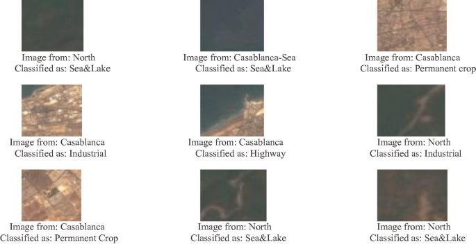
We aim to use the models we built during this work to construct a Moroccan LULC dataset. Indeed, we will choose one of these models to be used as an annotator of Moroccan satellite images. Therefore, we decided to test these classifiers’ ability to generalize to images of Moroccan regions. In this appendix we present the classification results of the four classifiers (i.e. LULC-Net, VGG16, VGG16 + LR and DLEnsemble1). The nine images we tested our models on are of the city of Casablanca where Industrial, Residential, Sea & Lake and highway classes are present, and of the North of Morocco where classes such as Forest, Pasture, River and Annual Corp are present.
-
LULC-Net

-
VGG16
-
VGG16 + LR

-
DLEnsemble1


Rights and permissions
Copyright information
© 2021 Springer Nature Switzerland AG
About this paper

Cite this paper
Benbriqa, H., Abnane, I., Idri, A., Tabiti, K. (2021). Deep and Ensemble Learning Based Land Use and Land Cover Classification. In: Gervasi, O., et al. Computational Science and Its Applications – ICCSA 2021. ICCSA 2021. Lecture Notes in Computer Science(), vol 12951. Springer, Cham. https://doi.org/10.1007/978-3-030-86970-0_41
Download citation
DOI: https://doi.org/10.1007/978-3-030-86970-0_41
Published:
Publisher Name: Springer, Cham
Print ISBN: 978-3-030-86969-4
Online ISBN: 978-3-030-86970-0
eBook Packages: Computer ScienceComputer Science (R0)