
Abstract
Automatic control of electric vehicles (EVs) is challenging due to the presence of system parameter uncertainty and large variations of resistant load. On the other hand, human drivers, without any knowledge of vehicle dynamic model and control, can properly deal with these challenges, thanks to the experiences acquired via training and practice. As a consequence, human expertise-based intelligent controllers are of interest for EVs, in which fuzzy logic controller (FLC) is a promising candidate considering its model-free essence with soft-computing techniques offering flexibility and robustness to the control system. This chapter proposes an FLC for speed control of AC electrical motors including induction motor (IM) and interior permanent magnet (IPM) synchronous motor in EV applications. The FLC membership functions and rules are designed with value normalization that allows the developed controller able to be flexible when applied to a wide range of speed control applications. The proposed FLC is numerically validated via an EV model with system parameters based on a practical off-road vehicle platform of our laboratory. Critical testing scenarios are employed including vehicle mass variations and rolling resistance force due to different load-carrying and road conditions. The results reveal that regardless of these uncertainty and load fluctuations, the speed error is kept within a bound of 2.5% comparing to the nominal speed of 40 km/h. The merit and flexibility of the proposed FLC have been discussed in comparison with the traditional PI controller and also with simulation on other platforms, i-MiEV of Mitsubishi in our lab. Moreover, thanks to its normalized design, the proposed FLC is not limited to the studied EVs, but can be applied to other e-mobility systems.
Access provided by Autonomous University of Puebla. Download chapter PDF
1 Introduction
The purpose of this chapter is to discuss an intelligent control technique based on fuzzy logic to improve the performance of motor drives in electric vehicle (EV) applications. The fundamental and the most distinguish feature of an EV compared to an internal combustion engine (ICE) car resides in the use of electric motor as “horse power,” which has clear advantages over its counterpart [1]:
-
The torque response of the electric motor is very accurate and quick, approximately 10-100 times faster than that of an ICE.
-
As the electromagnetic torque is proportional to the motor current, the developed torque can be calculated easily for the control purpose.
-
The use of electric motor allows eliminating many mechanical parts and enables various configurations, including attaching motor to each wheel, which allow flexible and advanced control algorithms to make car operation safer, more comfortable, and more intelligent.
Although several kinds of electric motors can be utilized, the recent battery electric vehicles (EVs) and hybrid electric vehicles (HEVs) primarily employ two types of motors: induction motors (IMs) and interior permanent magnet (IPM) synchronous motors. The control of these two motors will be addressed in this chapter.
Actually, motor drive is placed between the power electronic control layer (inner) and motion control (outer) in the traction architecture. Motor drive control consists of current control, flux control, and motor angular speed control. In the regular driving, the “speed controller” is the driver himself/herself, when he/she presses/releases the acceleration pedal to give the torque command signal to motor drive to attain the desired speed/travel trajectory. In the advanced EV control configuration, speed control is the inner loop of the motion control, for example, in the slip ratio control in [2], which enhances the safety and comfort of the driver and passengers. In other applications, the speed controller produces a close representation of how a human behaves during real-world driving exercises leading to a closer representation of how the final version of the vehicle will perform [3].
The design of the speed controller requires a special care, given the fact that there is an interaction of the environment to the vehicle body, such as road characteristics (surface adhesion, road slope), wind, etc. Besides, there are uncertainties in the system model caused by unknown or imprecise parameters during operation. All these disturbances and plant uncertainties have a direct affect to the performance of speed controller, especially when it was designed by model-based approach, such as proportional-integral-differential (PID) control.
Fuzzy logic (FL), which was first introduced by Zadeh on 1965 [4] as one class of artificial intelligence (AI), has been shown to be successfully applied to the motor drives in the industrial applications, transportation systems, aerospace, house appliances, etc. Fuzzy logic controller (FLC) for the speed control loop has been shown to have superior dynamic performance over PID speed controllers. FLC is a kind of nonlinear controller in its nature and has flexible control gains that can deal with ill-known model and disturbances [5]. In this chapter, the application of FLC in an EV will be extended by showing how it can control an IM or an IPM of any size and any configuration, with only minimal fine-tuning between different vehicle models.
After a review on recent applications of FLC to electric motor drives and EVs in Sect. 2, the modeling of an EV will be presented in Sect. 3, following by dynamic models of IM and IPM, as well as the vector control of the drives in Sect. 4. General procedure in the design of FLC is given in Sect. 5. The approach is applied in Sect. 6 to design an FL speed controller for an off-road EV. A comparative study with PI control is also provided. The EV has been adapted as an on-road laboratory platform for advanced electric and hybrid vehicle research at e-TESC Lab. of the University of Sherbrooke in Canada. The controlled system is tested by simulation in Sect. 7 with various scenarios for a performance analysis and evaluation. The flexibility of FLC is also demonstrated by employing the same FLC in other platform, the i-MiEV of Mitsubishi at CTI Laboratory for EVs, Hanoi University of Science and Technology in Vietnam. The summary of FLC design and its prospective will be given in the conclusion of this chapter.
2 Review on Recent Applications of FL to Motor Drives and EV Systems
Since its first engineering application was reported in 1975, fuzzy logic has been successfully used in numerous fields such as control systems engineering, image processing, power engineering, industrial automation, robotics, consumer electronics, and optimization. In electric motor drive areas in particular, extensive researches have been recognized since the 1990s. Applications include speed control of DC and AC drives, parameter estimation, diagnostics, and so on, for use in industrial processes, robotics, railway systems, photovoltaic (PV) renewable energy systems, etc. In the EVs/HEV domain, as the vehicle powertrain is electric motor drive, the experience on FLC design for industrial applications can be directly exploited. The fuzzy logic approach is especially suitable for EVs, considering high level of uncertainties and disturbance, such as road condition (tire-road friction, slope, slip/skid phenomena), wind, payload variation, etc.
In this section, a brief review on recent literature is carried out for FL in motor drives and EV applications.
FLC and adaptive FLC were used to improve the performance of induction motor drive [6, 7]. Experiment results with large variation of moment of inertia (as much as five times) showed that the robustness of the speed control system was greatly improved, compared to that of conventional PI control. The principle of FL was also utilized to estimate the rotor resistance, the parameter that has big influence on the accuracy of indirect vector control. FL utilization is found in a stator resistance observer of an IM in [8]. The current error is the input of the FLC process to decide the stator resistance increment. The estimated stator resistance is accepted in both simulated and experimental results.
FL can be used in the direct torque control configuration [9, 10]. Lai and Lin [9] presented a direct torque control based on a hybrid FLC for IM drive. The proposed technique alternates between PI controller and FLC controller by a simple switching mechanism, which is based on speed error as the threshold value. The PI controller works in steady state, while the FLC is selected in transient state to provide fast response and low overshoot. In comparison with other approaches, the hybrid fuzzy logic controller shows more robust performance and lowest root-mean-squared value of the speed error. In [10], a conventional PI or PID controller is replaced by a direct fuzzy logic for the torque regulation of an IM. The FLC requires the torque error and the torque error change as two inputs to calculate the incremental current command. It can be seen by the experimental results that this advanced method provides more accurate estimation of the torque and the flux than other techniques.
Sensorless speed vector control of an IM using model reference adaptive systems (MRAS) based on rotor flux is discussed in [11]. The conventional MRAS-PI speed estimator is replaced by two proposed controllers. The sliding mode control is employed to improve the stability performance and fast dynamic response; meanwhile, the speed error signal is minimized by the FL technique. In open-loop and closed-loop operation modes, the best performance is proved by MRAS-FLC in the transient and removed load torque disturbance conditions.
Liu et al. [12] introduce an expert controller based on fuzzy logic to improve the performance of the current controllers for IMs in field-weakening region. In high-speed flux-weakening of an IM, the expert controller treats the reference d-axis current \(i_{ds}^*\) from the flux-weakening (FW) strategy and the reference q-axis current \(i_{qs}^*\) from the speed regulator to handle the current change following two requirements: reasonable current tuning and limited current margin in FW. Compared with traditional current controllers, the command current pre-treated by the fuzzy inference expert controller has found an admissible trajectory for the current regulators.
A review of the different switching techniques and switching pattern of voltage space vectors, along with artificial intelligence controllers such as an artificial neural network, adaptive neural fuzzy inference system, and fuzzy logic control, has been made in [13].
Beside motor drives and power electronic control, FL has found many other energy-related applications in EV and HEV systems. Trovao et al. proposed an FLC as an energy management algorithm for multisource energy storage systems (MESSs) containing batteries and supercapacitors (SCs). One input of the FLC is the ratio between the power demanded by the powertrain and the rated power that the batteries can offer to the DC link; the other input is state of charge (SoC) of supercapacitors. The proposed FLC outputted the gain to decide the distribution ratio of the supercapacitor current in the MESSs [14, 15]. The coupled energy management algorithm based on FLC and filtering technique in the inner control layer can enhance the battery lifetime by reducing the battery current root mean square value by 12% in comparison with a battery-only architecture. The proposed energy management system (EMS), which is equivalent to an energy- and power-split management strategy, could enhance the stability of motor drive DC voltage [15] and has been tested on several EV configurations, including the three-wheel electric vehicle powered by battery-capacitor energy storage system [16].
In [17], by adopting the decision-making property of fuzzy logic, the driving map for an HEV is made according to driving conditions. An HEV, a city bus for shuttle service, with the proposed fuzzy logic-based driving strategy was built and tested at a real service route. It reveals the reduced NOx emission and better charge balance without an extra battery charger over the conventional deterministic table-based strategy.
Regarding the antilock braking systems of the electric vehicles, a wheel slip controller based on the fuzzy logic technique is proposed by Khatun in [18]. The torque demand is computed from the slip ratio, and the load torque. Over 5s of the examined period, the proposed fuzzy logic controller demonstrates a longitudinal performance enhancement even in the icy road condition. Power optimization can be achieved by using FLC [19]. The paper proposes an algorithm that reduces core losses of the induction motor, thus improving the efficiency of the driving system for electric vehicles.
Beside the applications to the energy management and traction system, FL approach has found in many topics of the automotive aspects such as driver assistance system, vehicle dynamic control and ride comfort, estimation of battery performance and battery changing, and so on. A good list of reference can be found in [20].
3 Vehicle Modeling
There exist various types of EV prototypes, such as the three-wheel EV [16], six-wheel EV [21], and eight-wheel EV driven by in-wheel motors [22]. As illustrated in Fig. 1, this chapter investigates one of the most popular four-wheel EV prototypes with front wheel drive. The AC motor M (IM or IPM motor in this chapter) converses electric power received from the storage system into the mechanical power in the form of electromagnetic torque T m in the motor shaft and rotor (mechanical) rotation speed Ω m. Gearbox GB is used to increase the torque generated by the motor by the gear ratio k gear. The torque is transmitted to the axle of the two front wheels, while the two rear wheels rotate freely under the effect of road friction. The rotational motions of the motor and the wheels are expressed as
where J m and J w are motor inertia and wheel inertia, respectively. The wheel has the radius R wh, the rotational speed Ω w,i and the driving force F d,i. The interaction between the motor and the wheel is represented by the drive shaft torque T d,i . Let K d be the torsional stiffness of the drive shaft, T d,i is expressed as follows

Electric vehicle and its traction system
Let v veh be the longitudinal speed of the vehicle. The difference between the vehicle speed and the wheel speed is specified by the slip ratio
where ε is a small positive number to avoid division by zero. As can be seen from Fig. 1, there exists a nonlinear relationship between the driving force and the slip ratio. This relationship is commonly described by the “magic formula” [23]
where
where A i = μ i F z,i, F z,i is the vertical load of the wheel i, μ i is the friction coefficient, and B i, C i, and D i are the shape factors. Summing all driving forces and resistance forces to the vehicle body of mass M veh, the longitudinal motion of the vehicle is given by the following equation:
The resistance forces act on the vehicle include air resistance, rolling resistance, and gravity component in the direction of travel when the vehicle is in climbing mode:
where f roll is the rolling resistance coefficient, g is the acceleration of gravity, α is the incline angle of the road, ρ is the mass density of the air, C d is the aerodynamic drag coefficient, A f is the equivalent frontal area of the vehicle, and v wind is the wind speed, which has the positive sign if the wind is resisting the forward motion of the vehicle and the negative sign if the wind pushes the vehicle forward.
To conclude this section, readers should notice that the set of Eqs. (1)–(8) describes a nonlinear complex system with several uncertainties. The common uncertainties are introduced by vehicle mass, wind force, and road incline angle. Moreover, the road condition might change frequently during the operation of the vehicle. Therefore, road friction coefficient and the shape factors of the magic formula are actually time-varying parameters. Also, the torsional characteristics of the shaft might introduce shaking vibration to the traction system [24]. Due to the above reasons, the complexity and burden of system design would be increased by several approaches such as pole placement, H-infinity-based robust control, and linear quadratic regulator (LQR). To extend the application of EV, automotive engineers should pay attention to the design approach which is practically simple but effective. This motivates us to think about the application of fuzzy logic control.
4 Modeling and Vector Control of AC Motor Drives
Using the vector control principle, an AC motor can be analyzed and controlled like a separately excited DC motor for high-performance applications. The fundamental principle of the vector control (VC) is to model the motor in d-q synchronously rotating frame and to control the torque generating component of the stator current in the q-axis while maintaining or adjusting the flux-related component of the stator current in the d-axis. Firstly introduced by Hasse (in 1969) [25] and Blaschke (in 1972) [26], thanks to the development of power switches and sophisticated microprocessors, vector control has become the standard in industry and other application fields since several decades.
The vector control principle was initially developed for IM. The method was then utilized directly for synchronous motors (SM), including PM synchronous motors. In the following, the VC will be presented for IM and then used for IPM motor.
4.1 Referential Transformation
The transformation between three-phase stationary reference frame a-b-c and the synchronous frame d-q is realized by Park transformation:

In the above equation d, q, and 0 represent the components in the d-axis, q-axis, and zero sequence, respectively; a, b, and c represent the components in three-phase stationary reference frame, θ e is the rotor electrical position; and θ e = ω e t with ω e, is the synchronous (electrical) angular speed.
When the zero-sequence element is zero, the matrix of direct Park transformation is simplified as

And the inverse Park transformation matrix \(K_{Park}^{-1}\) has the form

4.2 Modeling of IM in d-q Frame
The electrical dynamic model of the IM can be expressed in the d-q frame as shown in (12)
where u ds, u qs, i ds, and i qs denote the voltage and current in the d-q frame transformed from a-b-c frame; L s, L r, and L m are the stator, rotor, and magnetization inductance, respectively; R s and R r are the stator and rotor resistance; ψ dr is the d-axis rotor flux; and σ is the total linkage factor
Denote e d and e q the coupling terms
we can have compact form
The relation of synchronously rotating speed ω e and rotor electrical speed ω m is
where ω sl is the slip frequency and τ r is electrical time constant of rotor (τ r = L r∕R r).
The rotor position θ e needed in the Park transformation can be deduced from ω e as
The electromagnetic torque is generated by cross product of rotor flux and stator current and can be expressed in d-q frame:
To complete model of IM, we should include the dynamic equation of the rotating part:
where p is the number of pole pairs, Ω m is mechanical rotor speed (i.e., ω m = Ω m p), J eq is the equivalent moment of inertia, and T l is the equivalent load torque of the vehicle on the motor shaft. T l can be calculated from the vehicle model in Sec. 3, using (1)–(3) and (7), (8).
4.3 Vector Control of IM
If we orient the d-axis of the d-q frame to be coincided with the rotor flux vector, the flux component on the q-axis ψ qr is zero (where the name field-oriented control (FOC) method is originated), and (18) becomes
The torque developed by motor in (20) is proportional to the q-axis current i qs if the flux ψ dr is controlled to be constant. This important feature—the basic principle of vector control—shows the analogy of IM with DC motor with independent excitation.
The rotor flux can be dynamically estimated by Eq. (21):
In steady state, the flux is constant and becomes hence linear relation with current component i ds; therefore, (20) gives
4.4 Modeling of IPM Motors in d-q Frame
The modeling of IPM motors can be obtained in a similar way as for IMs. The electrical part model of the IPM motor is represented on the d-q coordinate system as follows:

where
-
R is the winding resistance
-
L d and L q the stator winding inductance in d and q axis, respectively
-
ψ p is the flux generated by the permanent magnet
The IPM motor model on the d-q frame is illustrated in Fig. 2. The interaction between the d and q axes in the electric part model (of the motor) is shown through the components

Block diagram of the structure of the IPM motor model on the d-q coordinate system
Equation (24) is equivalent to (14) in the case of IM. Eliminating coupling between the two d-q axes is one of the important problems in designing the motor controller in order to achieve good response of the motor torque to the torque demand.
The motor torque is given by
Equation (25) shows that the motor torque comprises of two parts: the mutual torque (as the result of interaction between the PM field and the stator current i q) and the reluctance torque.
The existence of the reluctance torque component is due to the difference between inductance L d and L q. It is the basis of the algorithm for optimal torque per current control, called maximum torque per ampere (MTPA) control, in order to exploit the saliency of the IPM motor.
4.5 General Layout of Vector Control of AC Motors
The modeling of IM and IPM motor, especially the torque expressions (20) and (25), leads to the similarity in the construction of control schema for both motors.
The general layout of vector control of AC motor is given in Fig. 3, in which we can see two control loops in the d-q frame: the inner loop for controlling the currents, the outer one for speed control in the q-axis and flux control in the d-axis. For the sake of simplicity in illustration of vector control, the decoupling networks based on (14) and (24) and the flux control loop are omitted in Fig. 3.

Principle schema of vector control of AC motor
If the bandwidth of the current control loops is high enough, the transfer function of the closed-loop current-controlled part is equivalent to a first-order function with a small time constant. We can then design the speed controller independent of current inner loops. The most popular control law is PI control, of which the gains are calculated using the motor parameters and equivalent parameters of the traction system.
Figure 4 presents the simplified block diagram of vector-controlled induction motor drives, in which the block “current-controlled part” includes the electrical part of the motor (Eqs. (14) and (15)) associated with two current controllers in Fig. 3. The (mechanical) rotational part of the motor is presented by the transfer function 1∕(J eq.s), which is directly deduced from (19). The motor speed controller is denoted C ω(s), and FW is the “flux-weakening” block.

Simplified block diagram of vector-controlled induction motor drives
The vector control of IPM motor can be described by the same manner, which results in the simplified block diagram as illustrated in Fig. 5.

Simplified block diagram of vector-controlled IPM motor drives
It is worth to note the particularity in the generation of current \(i_{ds}^*\) in d-axis path:
-
In IM drive, the reference value of the flux generating current component \(i_{ds}^*\) is kept constant under base speed and reduced inversely proportional with the speed in high-speed region. It can be realized by the FW block in Fig. 4.
-
In IPM drive, the MTPA algorithm is employed to maximize the torque/current ratio, by exploiting the saliency of the motor. The MTPA algorithm is activated in whole region of base speed. In the high-speed range, when the flux weakening is needed to avoid the voltage saturation, the MTPA algorithm is compared with the FW condition to yield the optimal value of current \(i_{ds}^*\) [27]. This operation is carried out in the block “MTPA-FW” in Fig. 5.
In the next part of the chapter, the design of a speed controller C ω(s) in Figs. 4 and 5 using fuzzy logic is addressed.
5 Fuzzy Logic Control: Principles and Design Procedure
5.1 FLC vs. Conventional Control
The design of a conventional control system is normally based on the mathematical model of a plant. Figure 6 illustrates the basic feedback configuration of a control system, in which P(s) represents the transfer function (or the model, in general) of the plant, C(s) denotes the controller, and u, y, w, and e are the control signal, output signal, input signal, and error signal, respectively. If an accurate mathematical model P(s) is available with known parameters, a controller C(s) can be designed for the specified performance. Unfortunately, for complex processes and systems, such as cement plants, electrical power delivery systems, EVs, etc., a reasonably good mathematical model is difficult to find. On the other hand, the plant operator may have good experience for controlling the process.

Basic feedback configuration of a control system
For most practical systems, models are often ill-defined. Even if a plant model is well-known, there may be parameter variation problems. Very often, the model is multivariable and nonlinear, such as the dynamic model of an AC motor. Vector control in d-q frame presented in previous section can overcome this problem, but the accurate vector control is nearly impossible [5]. In indirect vector control, for instance, motor parameters may vary considerably that affect the perfect field orientation, conditioned by calculation synchronously rotating speed ω e and rotor position θ e in (16) and (17) for direct and inverse coordinate transformation.
To overcome such problems, various adaptive control techniques and online parameter identification algorithms have been investigated. Better control performances are obtained, in expense of control complexity and larger execution time. Fuzzy logic control, on the other hand, does not strictly need any mathematical model of the plant. It is based on plant operator experience. FLC is basically an adaptive and nonlinear control, which gives robust performance for a linear and nonlinear plant with parameter variation [5].
If the mathematical model is known, the FLC design becomes more convenient. We can take this advantage for preliminary calculation and simulation stage to shorten the control design procedure.
Figure 7 shows the analogy between the FLC and the conventional controller in Fig. 6. The FLC takes the same place as of traditional controller C(s) in this feedback configuration. One input is error e between the reference (desired) signal and system output response; the other one is the change in error ce. Studies have shown that for most control problems, these two inputs’ configuration is good enough to give high performance. FLC in Fig. 7 is equivalent to a PI controller, of which the proportional and integral gains are automatically adjusted according to the working conditions. That explains why an FLC yields superior performance to conventional PI control. Other variances, equivalent to P-type FLC or PID-type FLC, are also possible [5]; however, the mentioned PI-type FLC is by far the most popular.

Basic configuration of a system using fuzzy logic: FLC in place of general conventional controller C(s)
5.2 General Design Procedure of an FLC
Fuzzy control is basically a process that is based on a fuzzy inference system (FIS). The FIS is essentially a formulation of the mapping from a given input set to an output set using FL. An FIS consists of following steps [5]:
-
Fuzzification of input variables
-
Applications of fuzzy operators (AND, OR) in the IF (antecedent) part of the rule and implication from the antecedent to the consequent (THEN part of the rule)
-
Aggregation of the consequents across the rules
-
Defuzzification
By placing the FIS in the general configuration of the feedback control as illustrated in Fig. 7, we can deduce the structure of an FLC in the control system. The FLC in Fig. 8 contains three main blocks, F (fuzzification), I (inference), and D (defuzzification), along with other two functional blocks, integral and knowledge base, which are described in the following:

Structure of FLC
-
1.
Fuzzification
A fuzzy variable has value that is expressed by natural language. The role of this stage is to converse the deterministic values (non-fuzzy or crisp) into fuzzy values:
-
Identify the input and output variables and range of (crisp) values.
-
Define the universe of discourse of input and output fuzzy variables.
-
Introduce the fuzzy sets of the fuzzy variables corresponding to input(s) and output(s).
-
Choose the form of membership functions.
The first input to FLC is the error e(k) between the reference w(k) (desired value of output) and the system output y(k) (actual value), and the second input is the change of error ce(k) between two instants k and (k − 1). The following relation can be extracted in a discrete system at instant k:
$$\displaystyle \begin{aligned} e(k)=w(k)-y(k) \end{aligned} $$(26)$$\displaystyle \begin{aligned} ce(k)=e(k)-e(k-1) \end{aligned} $$(27)A membership function (MF) can have different shapes, such as triangular, trapezoidal, Gaussian curve, bell, sigmoid, etc. MFs can be represented by mathematical functions, segmented straight lines, and look-up tables. The simplest and most commonly used MF is the triangular-type, because it can be realized by straight lines or by a linear function in programming. It can be symmetrical or asymmetrical in shape.
-
-
2.
Inference
Inference is the heart of an FLC that contains the capability of simulating the human decisions and deduces (infers) the action of fuzzy control by utilizing the fuzzy implication and the inference rules in the FL:
-
Formulate the rules of type IF . . . THEN . . . by utilizing fuzzy operators (AND, OR, NOT) in the IF (antecedent) part of the rule and implicating from the antecedent to the consequent (THEN part of the rule).
-
Establish the rule table (matrix).
-
Aggregation of the consequents across the rules.
There are a number of implication methods in the literature, of which the Mamdani type and Sugeno type are the most frequent. In the Mamdani method, each rule is evaluated by Minimum operator, and the total fuzzy output is the union (OR) of all the component MFs (Maximum operator). In the Sugeno (or Takagi-Sugeno-Kang) method of implication, output MFs are only constants or have linear relations with the inputs. With a constant output MF, it is defined as the zero-order Sugeno method, whereas with a linear relation, it is known as the first-order Sugeno method. It can be shown that if the Mamdani and Sugeno methods are applied to the same problem, the output is nearly the same. In practice, the Mamdani (or Max-Min method) is the most commonly used implication (aggregation) method.
-
-
3.
Defuzzification
The result of the implication and aggregation steps is the fuzzy output, which is the union of all the output of individual rules that are validated. Conversion of this fuzzy output to the crisp output is performed in this stage of defuzzification.
There are three methods of defuzzification: center of gravity method (COG), height method, and mean of maxima method.
In the center of gravity method of defuzzification, the crisp output Y O of the output fuzzy variable Y is taken to be the geometric center of the output fuzzy value μ(Y ) area, which is formed by taking the union of all the contributions of rules.
Mathematically, the COG can be expressed as follows
$$\displaystyle \begin{aligned} Y_O=\frac{\int Y.\mu(Y).dY}{\int \mu(Y).dY} \end{aligned} $$(28a)\(\int \mu (Y).dY\) denotes the area of the region bounded by the curve μ(Y ).
If the μ(Y ) is defined with a discrete membership function, the Y O can be calculated by following formula which uses summations instead of integrations.
$$\displaystyle \begin{aligned} Y_O=\frac{\sum^{n}_{i=1}Y_{i}.\mu(Y_{i})}{\sum^{n}_{i=1}\mu(Y_i)} \end{aligned} $$(28b)Here Y i is a sample element and n represents the number of contributed samples in the given fuzzy set.
In the height method of defuzzification, the COG method is simplified to consider only the height of each contributing MF and the midpoint of the base.
The height method of defuzzification is further simplified in the mean of maxima method, where only the highest MF component in the output is considered.
The COG method of defuzzification gives the most precise output value, with nearly similar calculation effort as other two methods. It is therefore the most utilized in literature.
-
4.
Integral
The output of FLC is the change (increment/decrement) of control variable. This signal is summed or integrated to generate the actual signal u to controlled plant.
In a discrete system, the updated control variable is calculated at instant k as
$$\displaystyle \begin{aligned} u(k)=u(k-1)+cu(k) \end{aligned} $$(29)That means the discrete integration is the sum of the change in control variable and its immediately past value.
-
5.
Knowledge base
The knowledge base block contains the database for the blocks F, I, and D and rule base for the I. In this meaning, the knowledge base block plays the role of supervision, which has a relation with the human intelligence (such as knowledge on the system and/or operation experience).
In the general structure of a fuzzy feedback control system in Fig. 8, the scale factors are introduced. The loop error e and the change in error ce signals are converted to the respective per unit signals by multiplying by the respective scale factors k e and k ce. Similarly, the output signal u is derived by multiplying the per unit (pu) output by the scale factor k ce and then summed to generate the u signal:
$$\displaystyle \begin{aligned} k_e=\dfrac{E}{e}; \qquad k_{ce}=\dfrac{CE}{ce}; \qquad k_{cu}=\dfrac{cu}{CU} \end{aligned} $$(30)Working with pu values presents a great advantage that the “normalized FLC” can be applied to all the plants of the same family. For other different plant, we only need to change the scale factors to conform to specific database. Besides, it becomes convenient to design the FLC. The scale factors can be constant or programmable. Programmable scale factors can control the operation sensitivity in different regions of control or the same strategy can be applied in similar response loops.
The above general design procedure will be illustrated by the design of an FLC for an off-road electric vehicle, driven by an IM.
6 Fuzzy Logic Speed Control for EV Applications
6.1 System Description
The design of FLC is demonstrated in the case study using eCommander off-road EV available at our laboratory at the University of Sherbrooke (Fig. 9). The EV has been adapted as an on-road laboratory platform for advanced electric and hybrid vehicle research in our Lab [28, 29].

The eCommander off-road vehicle model reference at the e-TESC laboratory, University of Sherbrooke
The vehicle is driven by a three-phase induction motor with the DC bus power supplied by a battery pack. The main parameters of the vehicle, the motor are given in Table 1.
6.2 Design of FL Speed Control
Consider the FL speed controller in a vector control drive system, i.e., FLC in place of C ω(s) in Fig. 4, which correspond to Figs. 7 and 8. The controller observes the pattern of the speed loop error signal and correspondingly updates the output cu (\(ci_{qs}^*\)) so that the actual speed Ω m matches the command speed \(\varOmega _m^*\).
The design of FLC for speed loop is carried out by following the general procedure described in Sect. 5.2.
-
1.
Fuzzification
There are two input signals to the FLC, the error \(e = \varOmega _m^*-\varOmega _m\) and the change in error, ce, which is related to the derivative of error de∕dt. In a discrete system, de∕dt = ce∕T s where T s is the sampling time. With constant T s, ce is proportional to de∕dt. Figure 8 also illustrates how to calculate ce by using delay operator z −1.
The controller output cu (minuscule) in a vector control drive is the change of current \(ci_{qs}^*\) (Figs. 5, 7, and 8). This signal is summed or integrated to generate the control signal u (\(i_{qs}^*\) in this case).
According to the data given in Table 1 for the vehicle and motor, we can calculate the universe of discourse for the inputs (speed errors e and change in speed error ce) and the output cu (change of current \(ci_{qs}^*\)). We can define fuzzy sets (linguistic values) as follows:
-
Negative big (NB)
-
Negative medium (NM)
-
Negative small (NS)
-
Nearly zero (ZE)
-
Positive small (PS)
-
Positive medium (PM)
-
Positive big (PB)
For the reason of simplicity and for a better visual effect, the fuzzy sets can be further coded by levels using numbers from − 3 (for NB) to 3 (for PB).
Table 2 summarizes the universe of discourse of variables and distribution of fuzzy sets. Note that the given values in the table are for the motor side, as all the parameters and variables of the vehicles have been converted into the motor shaft.
Table 2 Distribution of fuzzy sets The universes of discourse of the input and output variables are converted in pu values and expressed by MFs as shown in Fig. 10. The MFs of triangular-type are asymmetrical because near the origin (steady state), the signals require more precision. All the MFs are balanced for positive and negative values of the variables.
Fig. 10 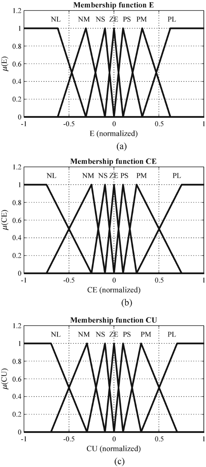
Membership functions of input and output variables. (a) Speed error membership function. (b) Change in speed error membership function. (c) Output membership function
-
-
2.
Inference
The rules of type IF…THEN are established in this stage. Given 7 fuzzy sets for each variable, there are 7 × 7 = 49 possible rules, which are connected by the operator OR:
-
Rule 1:IF e is (NB) AND ce is (NB) THEN cu is (NB)
-
OR
-
Rule 2: IF e is (NB) AND ce is (NM) THEN cu is (NB)
-
…
-
OR
-
Rule 49: IF e is (PB) AND ce is (PB) THEN cu is (PB)
Table 3 shows the corresponding table of rules for the speed controller, expressed in pu. The top row and left column of the matrix indicated the fuzzy sets of the variables E and CE, respectively, and the MFs of the output variable CU are shown in the body of the matrix. Note that the rule table is displayed by using the levels (− 3; 3) for the linguistic values.
Table 3 Rule table for FLC of speed control For a given operation point, only some rules are active, which are then implicated using Max-Min operators (Mamdani method of implication):
-
Calculate the degree of fulfillment (DOF) of each rule using the AND or min operator.
-
Aggregate the total fuzzy output using OR or max operator.
-
-
3.
Defuzzification
The crisp output CU, the change of q-axis current (pu) \(ci_{qs}^*\), is calculated by using (28b) of the the COG method:
$$\displaystyle \begin{aligned} Ci_{qs}^*=\frac{\sum_{i=1}^n Ci_{qs,i}^* .\mu(Ci_{qs,i}^*)}{\sum_{i=1}^{n}\mu(Ci_{qs,i}^*)} \end{aligned} $$(31)where \(\mu (Ci_{qs,i}^*)\) is the membership function of the \(Ci_{qs,i}^*\), i is a sample element and n represents the number of contributed samples in the given fuzzy set.
\(Ci_{qs}^\ast \) is then conversed by scale factor k cu to give the change of current \(ci_{qs}^*\). This signal is integrated to generate the control signal u (\(i_{qs}^*\) in this case).
Figure 11 shows the fuzzy surface of the rules from the rule table (matrix). It can be seen that the distribution is concentrated around the origin, meaning that high accuracy of the controlled system is expected.
Fig. 11 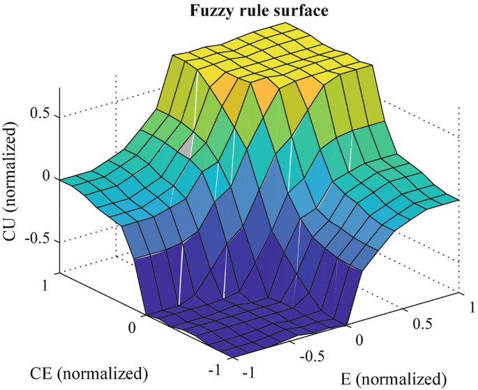
Fuzzy rule surface
The rule matrix and MF description of the variables are based on the knowledge of the system, and their fine-tuning may be time-consuming for optimal performance. For a simulation-based system design, controller tuning by the C-programming or recently with the help of the MATLAB Fuzzy Logic ToolboxTM, may be reasonably fast.


6.3 Comparison of PI Controller and FLC
6.3.1 Speed Control Using PI Controller
To control the speed of a motor, proportional-integral controller (PIC) has been shown to be a standard method. For instance, a traditional way to design the PIC-based speed control is as follows. We let the transfer function from motor torque to motor speed and the transfer function of the PIC be
where k p and k i are the control gains. The transfer function of the closed-loop system P c(s) including P m(s) and C m(s) is
Let λ 1 and λ 2 be the desired poles of P c(s), and the PI gains can be derived as
Readers should notice that the motor torque is limited by the maximum motor current. On the other hand, the current control loop always has a certain bandwidth. Therefore, λ 1 and λ 2 must not be placed too far from the origin in the left half-plane.
6.3.2 Preliminary Discussion
The above design procedure works really well if we only control a separate motor drive. However, the circumstance changes considerably when dealing with the application of EVs with the model shown in Fig. 1. The targeted plant consists of the EV body, the motor, and the mechanism that connects them. The EV plant is actually nonlinear. Hence, the nominal transfer function (32) fails to describe the true dynamics of the targeted plant. The designers also suffer from physical uncertainties, such as the vehicle mass, the road friction coefficient, and the torsional stiffness of the drive shaft. Considering the aforementioned issues, the disadvantages of PIC for EV have been discussed in our recent studies [30, 31]. Although stable poles are placed to the local transfer function P c(s), the poles of the overall system might change their place during long-term operation of EV. If the poles move toward the imaginary axis, the control system might suffer from vibration. Some robust control tools can improve system performance, and the typical tool is disturbance observer (DOB) [32]. Although DOB is simple to be implemented, its design and analysis are nontrivial for a nonlinear system as EV. The design of DOB requires several techniques as H-infinity norm and μ-synthesis. From practical point of view, automotive engineers still need some approaches which are convenient to design without using complex calculations.
Based on the above discussion, FLC turns out to be an attractive candidate for speed control. Following the previous section, readers can see that actually the FLC consists of two actions: the integral control action and the proportional control action. However, unlike the traditional fixed-gain PIC, FLC can be treated as a PIC with the gain adjusted and refined in real time by the fuzzy law.
7 Simulation and Performance Evaluation
7.1 Comparative Study of PI Controller and FLC
To compare the performance of PIC and FLC, we considered the motor speed control problem described in Fig. 4 and assume that the reference speed is given when the vehicle runs on the road surface with the friction coefficient μ = 0.8. The road friction coefficient was reduced to μ = 0.3 in the short period from 12 s to 14 s.
The PIC is designed using (35) with the desired poles λ 1,2 = −14 ± 6j, and the moment of inertia J eq is calculated using nominal mass of the vehicle. The nominal mass is calculated under the assumption that the vehicle has two passengers. The weight of each passenger is 70 kg.
Two test cases were performed. In Test 1, the plant is the simplified linear model (32). Both PIC and FLC showed very good control performances as can be seen in Fig. 12. In the Test 2, the above controllers were verified by using the nonlinear vehicle model described by Eqs. (1)–(8). In this test, the vehicle has to carry four passengers with the additional luggage of 50 kg. As can be seen from Fig. 13, both controllers still guarantee good tracking performances. However, the PIC has suffered from more oscillation with a higher overshoot. Motivated by the above results, in the following section, we have verified the performance of FLC and the overall control system in Fig. 4 by a standard driving cycle test.

Simulation results with simplified linear model without uncertainties. (a) Speed response. (b) Speed zoom

Simulation results (using nonlinear EV model with parameter uncertainties). (a) Speed response. (b) Speed zoom
7.2 Simulation of Vehicle Operation
In order to examine the performance, especially the robustness of the fuzzy logic speed controller, the vehicle is tested over the modified ECE cycle (to be suitable for the off-road vehicle speed range), the maximum speed of 45 km/h, and a duration of 195 s.
The fuzzy logic speed controller is realized by using the Fuzzy Logic ToolboxTM of MATLAB. Main results are reported in Fig. 14.

Vehicle speed response over the modified ECE driving cycle under system parameters and resistance variations. (a) Vehicle speed response. (b) Speed zoom 1. (c) Vehicle mass. (d) Speed zoom 2. (e) Rolling coefficient. (f) Speed zoom 3. (g) Motor torque. (h) Speed error
For system parameter variation, the vehicle total mass changes two times at the two stop periods (Fig. 14c). At the beginning, there is a 70-kg person driving the vehicle; then, at the 40th second, the vehicle is fully loaded with 272 kg of goods and two 70-kg people; finally, at the 100th second, the goods are unloaded. Consequently, the vehicle inertia characteristic changes during the driving cycle. Moreover, we examine the vehicle running on different road conditions with the rolling resistance coefficient varying from 0.02 to 0.08 as presented in Fig. 14e. The resistant force of the road to the vehicle is therefore significantly changed.
The global response given in Fig. 14a and the relative error (in comparison to the top speed of 40 km/h) plotted in Fig. 14h confirm the good performance of the vehicle speed fuzzy logic controller. Thanks to the fast torque dynamics of the electrical motor reflected in Fig. 14g, the controller can quickly respond to reference change and robustly adapt to the parameter and disturbance variations to keep the error always lower than 2.5%.
To have a better view, three areas of the speed response are zoomed in. Zoom 1 (Fig. 14a) shows the overshoot when the speed reference is set to 12 km/h and the speed drop when f roll suddenly raises from 0.035 to 0.06 with only a person driving the vehicle. In Zoom 2 plotted in Fig. 14b, when the vehicle is fully loaded and one more person added, the rolling resistance coefficient reduces to 0.02 that makes the speed raising higher than the reference. Finally, Zoom 3 presents the scenario that the coefficient f roll dramatically increases four times, from 0.02 to 0.08, which causes a drop of vehicle speed. At this time, the vehicle carries only two people as the goods were released at the previous stop period. In the all three scenarios, it can be seen that the fuzzy logic controller quickly responds to the resistant force alterations regardless of different vehicle total mass. The vehicle speed, after small errors due to the disturbance changes, is forced to follow the reference within about 1 s. That verifies the robustness of the developed fuzzy logic vehicle speed controller.
7.3 Flexibility of Fuzzy Logic Controller
The previous section shows that, in comparison with the traditional PIC, FLC might improve the performance of the motor actuator to a certain extent. This subsection is to discuss another merit of FLC, the flexibility. To this end, we demonstrate the performance of FLC using a completely different targeted plant. Figure 15 shows the commercial car Mitsubishi i-MiEV, which is acquired to serve as research prototype at the CTI Lab. for EVs, Hanoi University of Science and Technology, Vietnam. The measurement of the vehicle and motor parameters has been conducted in our Lab, and the values are reported in Table 4. In comparison with the eCommander in Fig. 9 and Table 1, the i-MiEV has heavier weight and driven by a different drivetrain with IPM motor.

Mitsubishi i-MiEV as research prototype at CTI Lab. for EVs, Hanoi University of Science and Technology
In this case study, we control the speed of the IPM motor attached to the i-MiEV vehicle. The test condition and the reference speed are similar to the previous test using the eCommander vehicle. In this test, we have treated the i-MiEV as if a “black box.” This means we assume we do not know the physical parameters of the i-MiEV. We have used the same FLC developed for the eCommander in Sect. 6 and only adjusted the gain k cu. As can be seen in Fig. 16, the tracking performance was poor if k cu is small. On the other hand, the motor speed suffers from vibration if we selected for k cu a really big value. This also results in the vibration to the motor torque (Fig. 17). Such vibrations should be eliminated since they reduce the comfort of the driver and introduce negative effects to the inner loop of the motor drive system (current control loop, power electronics converter control). The designer should compromise the trade-off between tracking performance and the driver comfort when adjusting the gain of the FLC.

Performance of fuzzy logic controller with different gains k cu. (a) Speed response. (b) Speed zoom

Motor torque with different gains k cu
This simulation study clarifies the flexibility of FLC for practical applications. After developing the fuzzy law using a given vehicle prototype (eCommander), the controller can be readily implemented for other vehicle prototypes. Even if the i-MiEV is a “black box,” we can quickly perform fine-tuning process to achieve a good control performance.
8 Conclusion
Electrification becomes an indispensable trend in automotive industry. While energy storage systems are the key components to enable EV penetration into the market, electric motors are the soul of the whole EV system. The use of electric motors not only does resolve the “traditional” problems of the pollution and fossil fuel shortage but also means many other features, such as safer, more comfortable, and more enjoyable to drive. As many latest technologies can be embedded, the vehicle can be autonomous and acts as an intelligent agent in the ecosystem of the Internet of Things and smart energy.
It is expected that modern EVs in the very future will be equipped by one of the five levels of autonomous driving. In the normal mode, the driver imposes the demand torque to the traction part by pressing/releasing the acceleration pedal. In the driver assistance mode (level 1), for instance, the vehicle can be monitored through cruise control. In the last case, the reference torque is generated by the vehicle speed control loop. This chapter devotes to designing the speed controller and has shown how we can incorporate FLC, a class of artificial intelligence, into the whole system.
Inspired by the advantages of an electric motor that make fundamental merits of EVs over ICE vehicles, the chapter focuses on how to design the “best quality” of the motor torque reference. The FLC approach has been adopted and utilized in a direct and simple way, but very systematic in the practical design point of view.
After a thorough literature review on fuzzy control applications for motor drives and EVs, the vehicle powertrain has been modeled focusing on the drivetrain and the electrical motor models. Standing out in other works dealing with a specific sort of traction drive, this chapter has figured out two commonly used AC motor drives for EVs, which are IM and IPM motor. These two kinds of motors can utilize the common general vector control layout. Afterward, the FLC principle and design procedure have been addressed from philosophy to detailed guideline.
A comparative study by simulation has shown that if the plant is of a simplified linear model, both PI controller and FLC yielded very good and similar control outcome, in terms of overshoot, response time, tracking error, and steady-state error. However, when considering the real model of EV with nonlinear characteristics, the FLC showed better performance than the PI controller.
The proposed FLC has been evaluated via numerical simulation using a practical vehicle-based model. To verify the robustness and uncertainty-tolerant ability of the fuzzy controller, both parameter and disturbance variations have been applied to the system. The results show that despite of up to 39% of vehicle mass change and 300% of rolling resistance force alteration, the tracking performance of the vehicle speed control loop is ensured with less than 2.5% of relative error.
Moreover, thanks to the normalization of the membership functions and inference design, the proposed FLC can tolerate a wide range of practical applications. It is tested by utilizing the same FLC for other EV platforms, the Mitsubishi i-MiEV driven by an IPM motor. The simulation study has confirmed the flexibility of the FLC for practical applications. A controller designed for a vehicle can be conveniently implemented for other vehicle prototypes. Only fine-tuning process is required to achieve a good control performance.
The principle of FLC can also be further applied in other control layers of the EV system. More uncertainty and nonlinearity such as slippery characteristics of tire dynamics would be also of interest for future studies based on this FLC.
References
Y. Hori, Future vehicle driven by electricity and control-research on four-wheel-motored UOT Electric March II. IEEE Trans. Ind. Electron. 5, 954–962 (2004)
H. Fujimoto, Regenerative brake and slip angle control of electric vehicle with in-wheel motor and active front steering. Tech. rep., SAE Technical Paper, 2011
S. Cash, O. Olatunbosun, Fuzzy logic field-oriented control of an induction motor and a permanent magnet synchronous motor for hybrid/electric vehicle traction applications. Int. J. Electric Hybrid Veh. 9(3), 269–284 (2017)
L.A. Zadeh, Fuzzy sets. Inform. Control 8(3), 338–353 (1965)
B.K. Bose, Modern Power Electronics and AC Drives (Prentice Hall, Englewood Cliffs, 2002)
M. Ta-Cao, H. Le-Huy, Model reference adaptive fuzzy controller and fuzzy estimator for high performance induction motor drives, in IEEE Industry Applications Conference—IAS’96, vol. 1 (1996), pp. 380–387
M. Ta-Cao, Digital Control of Induction Machines using Fuzzy Logic. Ph.D. Dissertation, Université Laval, 1997. Text in French
B. Karanayil, M.F. Rahman, C. Grantham, Stator and rotor resistance observers for induction motor drive using fuzzy logic and artificial neural networks. IEEE Trans. Energy Convers. 20(4), 771–780 (2005)
Y.-S. Lai, J.-C. Lin, New hybrid fuzzy controller for direct torque control induction motor drives. IEEE Trans. Power Electron. 18(5), 1211–1219 (2003)
H. Rehman, Fuzzy logic enhanced robust torque controlled induction motor drive system. IEE Proc. Control Theory Appl. 151(6), 754–762 (2004)
S.M. Gadoue, D. Giaouris, J.W. Finch, MRAS sensorless vector control of an induction motor using new sliding-mode and fuzzy-logic adaptation mechanisms. IEEE Trans. Energy Convers. 25(2), 394–402 (2009)
Y. Liu, J. Zhao, R. Wang, C. Huang, Performance improvement of induction motor current controllers in field-weakening region for electric vehicles. IEEE Trans. Power Electron 28(5), 2468–2482 (2012)
M.A. Hannan, J. Abd Ali, P.J. Ker, A. Mohamed, M.S. Lipu, A. Hussain, Switching techniques and intelligent controllers for induction motor drive: issues and recommendations. IEEE Access 6, 47489–47510 (2018)
J.P. Trovão, M.A. Silva, C.H. Antunes, M.R. Dubois, Stability enhancement of the motor drive DC input voltage of an electric vehicle using on-board hybrid energy storage systems. Appl. Energy 205, 244–259 (2017)
J.P. Trovão, M.A. Silva, M.R. Dubois, Coupled energy management algorithm for MESS in urban EV. IET Electr. Syst. Transp. 7(2), 125–134 (2017)
J.P.F. Trovão, M.-A. Roux, E. Ménard, M.R. Dubois, Energy- and power-split management of dual energy storage system for a three-wheel electric vehicle. IEEE Trans. Veh. Technol. 66(7), 5540–5550 (2017)
H.-D. Lee, S.-K. Sul, Fuzzy-logic-based torque control strategy for parallel-type hybrid electric vehicle. IEEE Trans. Ind. Electron. 45(4), 625–632 (1998)
P. Khatun, C.M. Bingham, N. Schofield, P. Mellor, Application of fuzzy control algorithms for electric vehicle antilock braking/traction control systems. IEEE Trans. Veh. Technol. 52(5), 1356–1364 (2003)
R. Kassem, K. Sayed, A. Kassem, R. Mostafa, Power optimisation scheme of induction motor using FLC for electric vehicle. IET Electr. Syst. Transp. 10(3), 301–309 (2020)
V. Ivanov, A review of fuzzy methods in automotive engineering applications. Eur. Transp. Res. Rev. 7(3), 1–10 (2015)
L. Boulon, D. Hissel, A. Bouscayrol, O. Pape, M. Péra, Simulation model of a military HEV with a highly redundant architecture. IEEE Trans. Veh. Technol. 59(6), 2654–2663 (2010)
S. Hiroshi, Multi-purpose electric vehicle “KAZ” . IATSS Res. 25(2), 96–97 (2001)
H.B. Pacejka, Tyre and Vehicle Dynamic (Elsevier BVl, 2006)
T. Karikomi, K. Itou, T. Okubo, S. Fujimoto, Development of the shaking vibration control for electric vehicles, in 2006 SICE-ICASE International Joint Conference (2006), pp. 2434–2439
K. Hasse, Zur Dynamik drehzahlgeregelter Antriebe mit stromrichtergespeisten Asynchron-Kurzschlusslaufermaschinen. Ph.D. Dissertation, Technische Hochschule Darmstadt, 1969. Text in German
F. Blaschke, The principle of field orientation as applied to the new transvector closed loop control system for rotating field machines. Siemens Rev. 34(3), 217–220 (1972)
K.H. Nam, AC Motor Control and Electrical Vehicle Applications (CRC Press, Boca Raton, 2019)
M.J. Blondin, J.P. Trovão, Soft-computing techniques for cruise controller tuning for an off-road electric vehicle. IET Electr. Syst. Transp. 9(4), 196–205 (2019)
C.T. Nguyen, B.-H. Nguyen, J.P.F. Trovão, M.C. Ta, Effect of battery voltage variation on electric vehicle performance driven by induction machine with optimal flux-weakening strategy. IET Electr. Syst. Transp. 10(4), 351–359 (2020)
B.-M. Nguyen, S. Hara, H. Fujimoto, Y. Hori, Slip control for IWM vehicles based on hierarchical LQR. Control Eng. Pract. 93, 104179 (2012)
B.-M. Nguyen, H.V. Nguyen, M. Ta-Cao, M. Kawanishi, Longitudinal modelling and control of in-wheel-motor electric vehicles as multi-agent systems. Energies 13(20), 5437 (2020)
T. Umeno, Y. Hori, Robust speed control of DC servomotors using modern two degrees-of-freedom controller design. Trans. Ind. Electron. 38(5), 363–368 (1991)
Acknowledgements
We would like to express our sincerest gratitude to Dr. Bảo-Huy Nguyê~n, postdoctoral researcher at e-TESC Lab., Department of Electrical and Computer Engineering, University of Sherbrooke, Canada, for his time contributing the simulations in Sects. 6.2 and 7.2. We also express our deepest thanks to Prof. João Pedro F. Trovão at e-TESC Lab., Department of Electrical and Computer Engineering, University of Sherbrooke, Sherbrooke, QC, J1K 2R1, Canada, for his discussion and his great support of the electric vehicle model used in this study.
Author information
Authors and Affiliations
Corresponding author
Editor information
Editors and Affiliations
Rights and permissions
Copyright information
© 2022 The Author(s), under exclusive license to Springer Nature Switzerland AG
About this chapter

Cite this chapter
Ta, M.C., Nguyen, BM., Vo-Duy, T. (2022). Fuzzy Logic Control for Motor Drive Performance Improvement in EV Applications. In: Blondin, M.J., Fernandes Trovão, J.P., Chaoui, H., Pardalos, P.M. (eds) Intelligent Control and Smart Energy Management. Springer Optimization and Its Applications, vol 181. Springer, Cham. https://doi.org/10.1007/978-3-030-84474-5_13
Download citation
DOI: https://doi.org/10.1007/978-3-030-84474-5_13
Published:
Publisher Name: Springer, Cham
Print ISBN: 978-3-030-84473-8
Online ISBN: 978-3-030-84474-5
eBook Packages: Mathematics and StatisticsMathematics and Statistics (R0)