Multidisciplinary System Modeling and Optimization

Abstract

With the increasing complexity of systems such as aerospace vehicles, it has become more and more necessary to adopt a global and integrated approach from the early steps and all along the design process. Tightly coupling aerodynamics, propulsion, structure, guidance and navigation, trajectory, etc. but also taking into account environmental and operational constraints as well as manufacturability, reliability, maintainability is a huge challenge.

1 Introduction

With the increasing complexity of systems such as aerospace vehicles, it has become more and more necessary to adopt a global and integrated approach from the early steps and all along the design process. Tightly coupling aerodynamics, propulsion, structure, guidance and navigation, trajectory, etc. but also taking into account environmental and operational constraints as well as manufacturability, reliability, maintainability is a huge challenge. For instance, for launch vehicle, it is typically considered that 80% of the life-cycle cost is locked in by early design decisions (Blair et al. 2001). The field of multidisciplinary design optimization (MDO) provides some answers on how to integrate more and more knowledge into the design process while reducing the design cycles. MDO can be thought as a set of engineering methods and tools to handle complex design problems involving several coupled disciplines. It consists of a core of key methodologies such as multidisciplinary problem formulations, optimization algorithms, surrogate-based high-fidelity tools, etc. which are validated and enriched through confrontation to various kinds of design studies. It provides an informed decision framework for the system designers. In the MDO formalism, a system is described as a set of interconnected subsystems (called disciplines) in order to model its dynamics and to estimate its performance. MDO approaches have been applied to a large panel of case studies in various fields such as aircraft (Henderson et al. 2012; Nguyen et al. 2013; Kenway et al. 2014), launch vehicles (Braun 1996; Balesdent et al. 2012; Breitkopf and Coelho 2013), spacecraft (Hwang et al. 2013; Huang et al. 2014), automotives (McAllister and Simpson 2003), ships (Peri and Campana 2003), buildings (Choudhary et al. 2005), etc. and offer methods to solve complex design optimizations which are laborious to handle with the classical design methods (Alexandrov 1997). Classical design approaches (Figure 1.1) consist of a sequence of discipline optimizations. However, in the case of complex system design, the disciplines often present antagonistic objectives and the classical design approaches have difficulty in the search for a compromise between these conflicting disciplinary objectives (Balesdent et al. 2012). For instance, in launch vehicle design, the aerodynamics discipline may tend to decrease the stage diameters to decrease the drag during the atmospheric flight, whereas the structure discipline may tend to increase it for stress and stability reasons. Some review articles (Agte et al. 2010; Alexandrov 1997; Balling and Sobieszczanski-Sobieski 1996; Sobieszczanski-Sobieski and Haftka 1997; Tosserams et al. 2009; Martins and Lambe 2013; Balesdent et al. 2012) provide a state of the art of the different MDO methods.

Fig. 1.1

Classical design approaches

Unlike the sequential disciplinary optimizations (Figure 1.1), in MDO, the interactions between the disciplines are directly taken into account (Balesdent et al. 2012) (Figure 1.2). Moreover, the design of complex systems requires diverse fields of expertise and with the globalization of the industries, it involves engineers distributed all over the world. The data exchange between the teams is a crucial point to take into account in the design process. MDO approaches aim to facilitate the discipline exchanges in order to find an optimal solution in reduced time and costs. The MDO formulations take advantage of the inherent synergies and couplings between the disciplines involved in the design process to decrease the computational cost and/or to improve the quality of the global optimal design (Sobieszczanski-Sobieski and Haftka 1997). However, the complexity of the problem is significantly increased by the simultaneous handling of all the disciplines and their interactions. To subdue the complexity introduced by MDO, various MDO formulations have been developed.

Fig. 1.2

Multidisciplinary design optimization

This chapter introduces the fundamental concepts, notations, and methods required to describe a MDO process without the presence of uncertainty. In Section 1.2, the concept of discipline and the general MDO formulation are introduced in addition to the appropriate notations to establish the preliminary bases. In Section 1.3, the methods to handle the interdisciplinary coupling handling are described. These approaches may be distinguished into different categories: coupled and decoupled approaches, and single and multi-level formulations. Section 1.4 presents an overview of the existing MDO formulations in order to describe their keys steps and to highlight their main advantages and drawbacks.

2 Mathematical Formulation of the General Deterministic Multidisciplinary Design Optimization (MDO) Problem

In MDO, a discipline i is modeled by a function c _i(⋅) taking design variables and input coupling variables as inputs and computing output coupling variables. A discipline i is illustrated in Figure 1.3.

Fig. 1.3

Discipline modeling

A general MDO problem can be formulated as follows (Balesdent et al. 2012):

$$\displaystyle \begin{aligned} \begin{array}{rcl} {} \text{min} &\displaystyle \;&\displaystyle f(\mathbf{z,y,x}) \end{array} \end{aligned} $$

(1.1)

$$\displaystyle \begin{aligned} \begin{array}{rcl} \text{w.r.t.} &\displaystyle \;&\displaystyle \mathbf{z}, \mathbf{y}, \mathbf{x} \\ \text{s.t.} &\displaystyle \;&\displaystyle \mathbf{g}(\mathbf{z,y,x}) \leq 0 \end{array} \end{aligned} $$

(1.2)

$$\displaystyle \begin{aligned} \begin{array}{rcl} &\displaystyle &\displaystyle \mathbf{h} (\mathbf{z,y,x})=0 \end{array} \end{aligned} $$

(1.3)

$$\displaystyle \begin{aligned} \begin{array}{rcl} {} &\displaystyle &\displaystyle \forall (i,j) \in \{1,\ldots ,N\}^2 \; i\neq j,\; {\mathbf{y}}_{ij}={\mathbf{c}}_{ij}({\mathbf{z}}_i,{\mathbf{y}}_{.i},{\mathbf{x}}_i) \end{array} \end{aligned} $$

(1.4)

$$\displaystyle \begin{aligned} \begin{array}{rcl} &\displaystyle &\displaystyle \forall i \in \{1,\ldots ,N\},\; {\mathbf{r}}_i({\mathbf{z}}_i,{\mathbf{y}}_{.i},{\mathbf{x}}_i)=0 \end{array} \end{aligned} $$

(1.5)

$$\displaystyle \begin{aligned} \begin{array}{rcl} {} &\displaystyle &\displaystyle \mathbf{z_{\min}} \leq \mathbf{z} \leq \mathbf{z_{\max}} \end{array} \end{aligned} $$

(1.6)

All the variables and functions are described in the following paragraphs. Three types of variables are involved in a deterministic MDO problem:

• z is the design variable vector. The design variables evolve all along the optimization process in order to find their optimal values with respect to the MDO problem (objective function and constraints). The design variables may be shared between several disciplines (noted z _sh) or specific to one discipline. For example, the design variables specific to the discipline i are noted $\bar {\mathbf {z}}_i$. We note ${\mathbf {z}}_i=\{\mathbf {z_{sh}},\bar {\mathbf {z}}_i\}$ the input design variable vector of the discipline i ∈{1, …, N} with N the number of disciplines and $\mathbf {z}=\bigcup _{i=1}^N {\mathbf {z}}_i$ without duplication. For instance, the typical design variables in a launch vehicle design problem are the stage diameters, the pressures in the combustion chambers, the propellant masses, the fairing geometry parameters, etc.

• x is the state variable vector. Unlike z, the state variables are not independent degrees of freedom but depend on the design variables, the coupling variables y and the state equations characterized by the residuals r(⋅). These variables are often defined by implicit relations that require specific numerical methods for solving complex industrial problems. For example, the guidance law (modeled, for instance, by pitch angle interpolation with respect to a set of way points) in a launch vehicle trajectory discipline has to be determined in order to ensure payload injection into orbit. The guidance law is often the result of an iterative process minimizing the discrepancy between the target orbit injection and the real orbit injection. In such a modeling, the pitch angle way points are state variables for the trajectory discipline and the discrepancy between the actual and target orbits is the residual r(⋅).

• In a multidisciplinary environment, the disciplines exchange coupling variables, y (Figure 1.4). The latter link the different disciplines to model the interactions between them. c _ij(z _i, y _.i, x _i) is a coupling function used to compute the output coupling variable vector which is calculated by the discipline i and input to the discipline j. y _.i stands for the vector of all the input coupling variables of the discipline i and y _ij is the input coupling variable vector which is input to the discipline j and output from the discipline i. We note $\mathbf {y}=\bigcup _{i=1}^N{\mathbf {y}}_{.i}=\bigcup _{i=1}^N{\mathbf {y}}_{i.}$ without duplication. From the design variables and the input coupling variables to the discipline i, the output coupling variables are computed with the coupling function: c _i.(z _i, y _.i, x _i) and y _i. = (y _i1, …, y _iN) is the vector of the outputs of the discipline i and the input coupling variable vector of all the other disciplines requiring this couplings as inputs. For example, the sizing discipline computes the aerospace vehicle dry mass which is transferred to the trajectory discipline for a simulation of the aerospace vehicle flight. Another example is the classical aerodynamics and structural analysis (Figure 1.5) (Coelho et al. 2009; El Majd et al. 2010; Kennedy and Martins 2014; Kenway et al. 2014). For an aircraft, this analysis involves coupled analyses between the aerodynamics discipline (which requires the aircraft geometry and the deformations) and the structure discipline (which requires the aerodynamics loads on the aircraft structure and especially the wings). For the coupled systems, it is important to keep in mind that their designs involve goals which are often conflicting with each other, for instance, reducing weight may lead to higher structural stresses.

  Fig. 1.4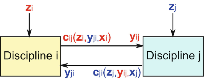

  

  Couplings between the discipline i and the discipline j

  Fig. 1.5

  

  Couplings between the aerodynamics and structure disciplines

In order to solve the MDO problem Equations (1.1–1.6), we are looking for:

• Inequality and equality constraint feasibility: the MDO solution has to satisfy the inequality constraints imposed by g(⋅) and the equality constraints imposed by h(⋅). These constraints translate the requirements for the system in terms of targeted performance, safety, flexibility, etc. For example, a target orbit altitude for a launch vehicle payload is an equality constraint that has to be satisfied.

• Individual disciplinary feasibility: the MDO solution has to ensure the disciplinary satisfaction through the equality constraints on the residuals r _i(⋅). The residuals r _i(⋅) quantify the satisfaction of the state equations in the discipline i. The state variables x _i are the roots of the state equations of the discipline i. For instance, the state equations may translate a thermodynamic equilibrium between the chemical components in the rocket engine combustion. In the rest of this chapter, it is assumed that the satisfaction of the disciplinary feasibility is ensured by the disciplines; therefore, no more references to the state variables and residuals will be done.

• Multidisciplinary feasibility: the MDO solution has to satisfy the interdisciplinary equality constraints (also referred to as multidisciplinary compatibility constraints) between the input coupling variable vector y and the output coupling variable vector which is the output of the coupling functions gathered in c(⋅) resulting from the discipline simulations. In two disciplines context, the couplings between the disciplines i and j are said to be satisfied (also called feasible, compatible, or consistent) when the following interdisciplinary system of equations is verified:

  $$\displaystyle \begin{aligned} \left\{ \begin{array}{c} {\mathbf{y}}_{ij}={\mathbf{c}}_{ij}({\mathbf{z}}_i,{\mathbf{y}}_{.i}) \\ {\mathbf{y}}_{ji}={\mathbf{c}}_{ji}({\mathbf{z}}_j,{\mathbf{y}}_{.j}). \end{array} \right. \end{aligned} $$

  (1.7)

  When all the couplings are satisfied, i.e. when Equations (1.7) are satisfied for all the couplings between all the disciplines, the system is said to be multidisciplinary feasible. The satisfaction of the interdisciplinary couplings is essential as it is a necessary condition for the modeled system to be physically realistic. Indeed, in the aerodynamics and structural example, if the aerodynamics discipline computes a load of 10 MPa, it is necessary that the structure discipline uses as input 10 MPa and not another value otherwise the coupled analysis is not consistent. The existing methods for the coupling satisfaction in the deterministic MDO are detailed in Section 1.3.

• Optimal MDO solution: f(⋅) is the objective function (also called performance) to be optimized. Multi-objective functions may be used to quantify several performances to be optimized (see Chapter 8). This kind of functions characterizes the system and is a measure of its quality expressed with some metrics (e.g., aerospace vehicle life cycle cost in euros, Gross Lift-Off Weight in kg, aircraft range in km). In general, the objective function has to be minimized.

To summarize, in order to solve a MDO problem, it is necessary to ensure:

• Requirement feasibility: respect of the requirements asked by the designer,

• Multidisciplinary feasibility: respect of the physical relevance for the obtained design,

• Individual disciplinary feasibility: respect of the disciplinary state equations,

• MDO solution optimality.

The multidisciplinary feasibility is a specificity of multidisciplinary systems which involve coupled analyses and require specific methodologies to guarantee it. The classical methods to ensure the interdisciplinary coupling satisfaction are detailed in the next section.

3 Multidisciplinary Coupling Satisfaction

In MDO, two categories of methods to satisfy the interdisciplinary couplings may be distinguished (Balling and Sobieszczanski-Sobieski 1996): the coupled approaches (Figure 1.6) and the decoupled approaches (Figure 1.7) and are introduced in this section.

Fig. 1.6

Multidisciplinary design optimization, coupled approach

Fig. 1.7

Multidisciplinary design optimization, decoupled approach

3.1 Coupled Approaches (Use of Multidisciplinary Analysis)

The coupled approaches (Figure 1.6) perform a multidisciplinary analysis (MDA) to ensure the interdisciplinary couplings at each iteration of the system-level optimization. MDA is an auxiliary analysis aiming to find an equilibrium between the disciplines by solving the system of interdisciplinary equations (Coelho et al. 2009). In other words, MDA consists in finding the value of the input coupling variables y satisfying the system of interdisciplinary equations (Equations 1.7). An iterative scheme is required to solve the system of equations because of the coupled nature of the disciplines. Two classical MDA methods are distinguished: either the Fixed Point Iteration (FPI) or an auxiliary optimization process minimizing the residuals of the interdisciplinary equations (Coelho et al. 2009; Breitkopf and Coelho 2013).

• Fixed Point Iteration. FPI is an iterative procedure involving a loop between the disciplines with no control on the coupling variables (excepted for the initialization) which directly results from the discipline simulations. Different schemes for iterative FPI exist in the literature. The most used are the Gauss–Seidel or the Jacobi approaches (Salkuyeh 2007; Lambe and Martins 2012; Martins and Lambe 2013) (Figure 1.9). FPI with the Gauss–Seidel scheme consists in successively analyzing the different disciplines with the updated output coupling variables from the disciplines computed previously. This FPI scheme can be interpreted as a generalized Gauss–Seidel scheme for multidisciplinary analysis because of its links with the Gauss–Seidel algorithm for solving linear algebraic equations. The Jacobi scheme differs from the Gauss–Seidel approach in the sense that the disciplines take as inputs the values of the coupling variables given at the previous Jacobi iteration. In that sense, in a Jacobi scheme, all the disciplines can be evaluated in parallel. It is important to note that FPI may not always converge, a theoretical analysis of conditions under which convergence can be guaranteed (for instance, if the interdisciplinary set of equations defines a contraction mapping) may be found in Ortega (1973). In the FPI approach, only one coupling vector is initialized (for instance, y _ij in Figure 1.8). The FPI algorithm for a scalar coupling variable between two disciplines is described in Algorithm 1 for the Gauss–Seidel scheme and in Algorithm 2 for the Jacobi scheme. These algorithms can be generalized to vector couplings and problems with more than two disciplines.

  Fig. 1.8

  

  General principle of FPI between the discipline i and the discipline j

  Fig. 1.9

  

  Gauss–Seidel vs Jacobi schemes for FPI between the discipline i and the discipline j. (a) Gauss–Seidel scheme for FPI between the discipline i and the discipline j. (b) Jacobi scheme for FPI between the discipline i and the discipline j

  Algorithm 1: FPI algorithm (Gauss–Seidel type) for scalar coupling between two disciplines

  

  Algorithm 2: FPI algorithm (Jacobi type) for scalar coupling between two disciplines

  

• Discrepancy minimization. Alternatively, MDA may be solved by minimizing the discrepancy between the input coupling variable vector and the coupling output vector (Tedford and Martins 2006) (Figure 1.10):

  $$\displaystyle \begin{aligned} \begin{array}{rcl} {} \text{min} &\displaystyle \;&\displaystyle \parallel{\mathbf{y}}_{1.}-{\mathbf{c}}_{1.}(\mathbf{z,y}_{.1})\parallel ^2+\cdots+\parallel{\mathbf{y}}_{N.}-{\mathbf{c}}_{N.}(\mathbf{z,y}_{.N})\parallel ^2 \\ \text{w.r.t.} &\displaystyle \;&\displaystyle \mathbf{y} \end{array} \end{aligned} $$

  (1.8)

  with y _i. the input coupling variable vector of all the disciplines linked to the discipline i. The interdisciplinary coupling system is solved when the optimizer converges such that the discrepancy is equal to zero. An efficient auxiliary optimization algorithm often requires fewer calls to the discipline i than FPI, as the optimization process chooses the steps more freely than FPI (Sankararaman and Mahadevan 2012). Newton–Raphson or staggered solution approaches (Felippa et al. 2001) are examples of root finding algorithms applied to MDA. More details on MDA can be found in Keane and Nair (2005). It is important to notice that the MDO formulations satisfying the interdisciplinary equations with MDA ensure the system feasibility at each system-level optimization iteration.

  Fig. 1.10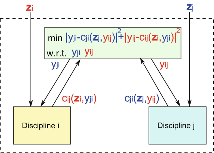

  

  Discrepancy minimization for the discipline i and the discipline j

It is worth noting that whatever the numerical scheme used to solve MDA, it is possible that the final couplings may depend on the initial guess. Indeed, a nonlinear system may have multiple equilibrium points resulting in several couplings satisfying the multidisciplinary feasibility. Even though such situations are rarely encountered in the aerospace vehicle design, MDA must be performed carefully to ensure that the most physically meaningful solution is picked.

3.2 Decoupled Approaches

The decoupled approaches (Figure 1.7) aim at removing MDA and at imposing equality constraints on the coupling variables in the MDO formulation at the system-level (Equation 1.4) to ensure the interdisciplinary coupling satisfaction only for the optimal design. Instead of solving the system of interdisciplinary equations at each of the MDO process iteration in z, equality constraints may be imposed between the input and the output coupling variables in the MDO formulation at the same level as the constraints g(⋅) and h(⋅): ∀(i, j) ∈{1, …, N}² i ≠ j, y _ij = c _ij(z _i, y _.i). These constraints impose to the optimal design the multidisciplinary feasibility. The basic idea is to define the input coupling variables y as optimization variables along with the design variables z. Indeed, in the decoupled approaches, the system-level optimizer controls both the design variables and the input coupling variables. Hence, the additional degrees of freedom introduced by expanding the variables handled by the system-level optimizer are controlled by the coupling equality constraints. The equality constraints on coupling variables may not be satisfied at each iteration but guide the search of optimal design.

The coupled and decoupled approaches to handle the interdisciplinary couplings have been incorporated in various MDO formulations that are briefly presented in the following sections.

4 MDO Formulations

A lot of MDO formulations have been proposed in the literature to efficiently solve general and specific engineering problems. Some articles (Balling and Sobieszczanski-Sobieski 1996; Alexandrov 1997; Balesdent et al. 2012; Martins and Lambe 2013; Breitkopf and Coelho 2013) provide a review of the different methods and compare them qualitatively and numerically on a benchmark of MDO problems (Yi et al. 2008; Tedford and Martins 2010).

This section presents the main MDO formulations that will be used in the following chapters. Classical MDO formulations may be classified in four categories (Figure 1.11) according to the coupled or decoupled and to the single or multi-level approaches:

• Single-level approaches with the use of MDA: e.g. MultiDiscipline Feasible (MDF) (Balling and Sobieszczanski-Sobieski 1996),

  Fig. 1.11

  

  Classification of the main MDO formulations

• Multi-level approaches with the use of MDA: e.g. Concurrent SubSpace Optimization (CSSO) (Sobieszczanski-Sobieski 1988), Bi-Level Integrated System Synthesis (BLISS) (Sobieszczanski-Sobieski et al. 1998),

• Single-level approaches with equality constraints on the coupling variables: e.g. Individual Discipline Feasible (IDF) (Balling and Sobieszczanski-Sobieski 1996), All At Once (AAO) (Balling and Sobieszczanski-Sobieski 1996),

• Multi-level approaches with equality constraints on the coupling variables: e.g. Collaborative Optimization (CO) (Braun 1996), Analytical Target Cascading (ATC) (Allison et al. 2005), Quasi Separable Decomposition (QSD) (Haftka and Watson 2005).

The single-level vs. multi-level formulations differ by the number of optimizers. Single-level formulations have only one system optimizer to solve the MDO problem, whereas in multi-level formulations, in addition to the system optimizer, the discipline (or subsystem) optimizers are introduced in order to distribute the problem complexity over the different dedicated discipline optimizations. Among the formulations relying on MDA, MDF is the most used (Balesdent et al. 2012). MDF is a single-level optimization formulation in which the system performance is evaluated with a disciplinary iterative process. CSSO and BLISS use MDA to ensure the interdisciplinary couplings but enable the decoupled discipline optimizations. IDF, CO, ATC, and AAO are fully decoupled formulations with the satisfaction of the couplings by incorporating additional variables and equality constraints in the formulations. The decoupled MDO formulations offer several advantages compared to MDF (Balesdent et al. 2012; Martins and Lambe 2013):

• The system-level optimization process allows parallel analyses of the disciplines; however, the load balancing has to be taken into account when some analyses or optimizations are much more expensive than others, such as in multi-fidelity optimization problems. For example, in Zadeh and Toropov (2002) the decoupled approaches are not efficient because of the inactivity of the processors running the inexpensive analyses and optimizations which is waiting for the updates from the other processors.

• The number of calls to the computationally expensive discipline codes may be notably decreased by avoiding expensive MDA calculations,

• The multi-level methods facilitate the system optimization by distributing the problem complexity over the different dedicated discipline optimizations. However, poor convergence rate may be observed due to the imbrication of several levels of optimization (DeMiguel and Murray 2000; Martins and Lambe 2013),

• In the multi-level approaches, the discipline optimizers handle the local design variables (decreasing the system-level design space size) and the system-level optimizer only controls the shared design variables between the disciplines and the coupling variables. Different suited optimizer algorithms may be used to solve the lower-level optimization problems.

However, compared to MDF, the decoupled MDO formulations require an appropriate interdisciplinary coupling handling and involve an optimization problem with more variables in total (the design variables and the coupling variables that can be distributed among the system and the local disciplinary optimizers in the case of multi-level approaches) and more constraints. In the next sections, two single-level formulations (one coupled and one decoupled) and four multi-level formulations (two coupled and two decoupled) are presented in order to highlight the coupling handling approaches in the main MDO formulations. First, the two single-level approaches are introduced.

4.1 MultiDiscipline Feasible (MDF)

The Multidiscipline Feasible (MDF) formulation (Figure 1.12) is the most used MDO method. This approach is described in Cramer et al. (1994) and Balling and Sobieszczanski-Sobieski (1996). MDF is a single-level coupled deterministic approach which uses MDA to ensure the interdisciplinary coupling satisfaction at each iteration of the system-level optimizer. Once the MDA is performed, the design variables and the converged values of the coupling variables are used to compute the objective function and the constraints. The disciplines are in charge of finding the state variable values satisfying the state equations consequently they do not intervene in the MDF formulation.

$$\displaystyle \begin{aligned} \begin{array}{rcl} {} \text{min} &\displaystyle \;&\displaystyle f\left(\mathbf{z},\mathbf{y}(\mathbf{z})\right) \end{array} \end{aligned} $$

(1.9)

$$\displaystyle \begin{aligned} \begin{array}{rcl} \text{w.r.t.} &\displaystyle \;&\displaystyle \mathbf{z} \\ \text{s.t.} &\displaystyle \;&\displaystyle \mathbf{g}\left(\mathbf{z},\mathbf{y}(\mathbf{z})\right) \leq 0 \end{array} \end{aligned} $$

(1.10)

$$\displaystyle \begin{aligned} \begin{array}{rcl} &\displaystyle &\displaystyle \mathbf{h} \left(\mathbf{z},\mathbf{y}(\mathbf{z})\right)=0 \end{array} \end{aligned} $$

(1.11)

$$\displaystyle \begin{aligned} \begin{array}{rcl} &\displaystyle &\displaystyle \mathbf{z_{\min}} \leq \mathbf{z} \leq \mathbf{z_{\max}} \end{array} \end{aligned} $$

(1.12)

with y(z) the (converged) coupling variable vector satisfying the system of interdisciplinary equations (could also be noted y ^FPI(z)) (Equations 1.7). It is important to notice that, in MDF, due to the repeated calls to MDA, at each iteration, each candidate solution is multidisciplinary feasible. The main advantage of MDF is its simplicity of implementation which involves only one system optimizer and MDA controls the interdisciplinary couplings. Moreover, this formulation is general enough to be easily adapted to all types of multidisciplinary systems. MDF is often considered as a reference due to its intrinsic interdisciplinary coupling satisfaction thanks to MDA. However, MDF presents also important drawbacks. MDA requires iterative loops between the disciplines and can be, therefore, computationally expensive. In the presence of computationally expensive disciplines, the repeated calls to MDA in MDF result in a prohibitive computational cost.

Fig. 1.12

MDF formulation

For large scale industrial design problems, each subsystem may involve specialists and engineering teams distributed all over the world and performing MDA becomes a complicated task as it requires (Balesdent 2011):

• the definition of each subsystem autonomy and domain of action with respect to all the involved collaborators,

• the management of the exchanges of information and data transmissions between the different subsystems,

• the traceability of the exchanged information and the evaluated system design.

Moreover, the subsystem analyses are performed sequentially and each team has to wait for the previous one in order to perform its tasks (when FPI with Gauss–Seidel is used to solve MDA) which can be very time consuming.

4.2 Individual Discipline Feasible (IDF)

Individual Discipline Feasible (Cramer et al. 1994; Balling and Sobieszczanski-Sobieski 1996) (Figure 1.13) is a decoupled single-level deterministic formulation (Equations 1.13–1.17). It replaces the computationally expensive MDA by introducing additional degrees of freedom, the input coupling variables controlled at the system-level, and by adding interdisciplinary coupling constraints in the formulation (Equation 1.16):

$$\displaystyle \begin{aligned} \begin{array}{rcl} {} \text{min} &\displaystyle \;&\displaystyle f\left(\mathbf{z},\mathbf{y}\right) \end{array} \end{aligned} $$

(1.13)

$$\displaystyle \begin{aligned} \begin{array}{rcl} \text{w.r.t.} &\displaystyle \;&\displaystyle \mathbf{z},\mathbf{y} \\ \text{s.t.} &\displaystyle \;&\displaystyle \mathbf{g}\left(\mathbf{z},\mathbf{y}\right) \leq 0 \end{array} \end{aligned} $$

(1.14)

$$\displaystyle \begin{aligned} \begin{array}{rcl} &\displaystyle &\displaystyle \mathbf{h} \left(\mathbf{z},\mathbf{y}\right)=0 \end{array} \end{aligned} $$

(1.15)

$$\displaystyle \begin{aligned} \begin{array}{rcl} {} &\displaystyle &\displaystyle \forall(i,j)\in\{1,\ldots,N\}^2 i\neq j, {\mathbf{y}}_{ij}={\mathbf{c}}_{ij}({\mathbf{z}}_i,{\mathbf{y}}_{.i}) \end{array} \end{aligned} $$

(1.16)

$$\displaystyle \begin{aligned} \begin{array}{rcl} &\displaystyle &\displaystyle \mathbf{z_{\min}} \leq \mathbf{z} \leq \mathbf{z_{\max}}. {} \end{array} \end{aligned} $$

(1.17)

Fig. 1.13

IDF method

This formulation allows to split the main problem into several subproblems by removing MDA. The input coupling variables are controlled by the system-level optimizer allowing to decouple the disciplines and to evaluate them in parallel. The optimizer exchanges the coupling information with all the disciplines to coordinate them to a multidisciplinary feasible solution. In order to ensure the system consistency for the optimal solution, equality constraints (Equation 1.16) between the input and the output coupling variables are added compared to MDF formulation. In IDF, the multidisciplinary feasibility is ensured only at the MDO problem convergence and the intermediate optimization solution consistency is not guaranteed. This decomposition approach increases the number of decision variables controlled by the system-level optimizer but the computational cost may be improved thanks to the discipline parallelization. Unlike MDF, at each system-level iteration, only one call to the disciplines is carried out. For large scale applications, the management tasks are less restrictive than in MDF because each discipline only dialogues with the optimizer.

Multi-level approaches have been proposed in order to ease the system-level optimization by introducing dedicated subsystem-level optimizers. Two families of decoupled MDO formulations are discussed in the following sections. First, Collaborative Optimization (CO) and Analytical Target Cascading (ATC) decompositions which belong to decoupled multi-level formulations are detailed and then Bi-Level Integrated Systems Synthesis (BLISS) and Concurrent SubSpace Optimization (CSSO) which may be viewed as an hybrid form between coupled and decoupled approaches are discussed.

4.3 Collaborative Optimization (CO)

Collaborative Optimization (CO) (Braun 1996) is a decoupled bi-level deterministic formulation (Figure 1.14). This formulation has been developed to offer more autonomy to the subsystems to satisfy the interdisciplinary couplings. CO may be resumed as follows:

$$\displaystyle \begin{aligned} \begin{array}{rcl} {} \text{min} &\displaystyle \;&\displaystyle f\left(\mathbf{z},\mathbf{y}\right) \end{array} \end{aligned} $$

(1.18)

$$\displaystyle \begin{aligned} \begin{array}{rcl} \text{w.r.t.} &\displaystyle \;&\displaystyle \mathbf{z},\mathbf{y} \\ \text{s.t.} &\displaystyle \;&\displaystyle J_{i.}({\mathbf{z}}_i^*,{\mathbf{z}}_i,\mathbf{y})=0, \forall i \in \{1,\ldots,N\} \end{array} \end{aligned} $$

(1.19)

$$\displaystyle \begin{aligned} \begin{array}{rcl} &\displaystyle &\displaystyle \mathbf{z_{\min}} \leq \mathbf{z} \leq \mathbf{z_{\max}} \end{array} \end{aligned} $$

(1.20)

with J _i. the optimized objective function of the ith discipline and z ^∗ the local copies of z controlled by the subsystem optimizer. The ith subsystem optimization problem is given by

$$\displaystyle \begin{aligned} \begin{array}{rcl} {} \text{min} &\displaystyle \;&\displaystyle J_{i.}=\parallel {\mathbf{z}}_i^*-{\mathbf{z}}_i \parallel^2_2 + \parallel {\mathbf{y}}_{i.}-{\mathbf{c}}_{i.}({\mathbf{y}}_{.i},{\mathbf{z}}_i^*) \parallel^2_2 \end{array} \end{aligned} $$

(1.21)

$$\displaystyle \begin{aligned} \begin{array}{rcl} \text{w.r.t.} &\displaystyle \;&\displaystyle {\mathbf{z}}_i^* \\ \text{s.t.} &\displaystyle \;&\displaystyle {\mathbf{g}}_i\left({\mathbf{z}}_i^*,{\mathbf{y}}_{.i}\right) \leq 0 \end{array} \end{aligned} $$

(1.22)

$$\displaystyle \begin{aligned} \begin{array}{rcl} &\displaystyle &\displaystyle \mathbf{h_i} \left({\mathbf{z}}_i^*,{\mathbf{y}}_{.i}\right)=0 \end{array} \end{aligned} $$

(1.23)

$$\displaystyle \begin{aligned} \begin{array}{rcl} &\displaystyle &\displaystyle {\mathbf{z}}_{i_{\mathbf{\min}}}^* \leq z^* \leq {\mathbf{z}}_{i_{\mathbf{max}}}^*. \end{array} \end{aligned} $$

(1.24)

Fig. 1.14

CO method

CO presents important advantages compared to the single-level MDO formulations. Indeed, CO allows to employ the most adapted optimization method to each discipline with possible actions of the disciplinary experts. Moreover, the design process offers modularity and flexibility to add or remove disciplines without modifying the entire design process. However, theoretical and practical convergence issues with respect to the quadratic constraint formulation have been observed by some researchers (Alexandrov and Lewis 2000) due to instabilities at the convergence. Several adaptations of CO have been proposed in order to overcome this difficulty (DeMiguel and Murray 2006). Nevertheless, this approach has been shown to provide good results for some MDO problems (Braun 1996).

4.4 Analytical Target Cascading (ATC)

The Analytical Target Cascading (ATC) method (Figure 1.15), described in Michelena et al. (1999, 2003) and Kim (2001), has been initially developed to formalize industrial product development processes. This formulation is adapted to solve problems with a hierarchical structure. ATC is a multi-level MDO method (possibly involving more than two levels) which hierarchically propagates system and subsystem-level targets through the different subsystem-levels. In this formulation, the initial problem is subdivided into a set of subproblems. The specified design targets are cascaded from the system-level to the lower-levels and are also rebalanced to the higher-levels after being optimized at the lower-levels.

Fig. 1.15

ATC method (Balesdent et al. 2012)

At each level of the design process, a specific optimization problem is formulated to minimize the errors between the level outputs and the propagated objectives, and thus to ensure the consistency concerning the couplings between the upper and lower optimization levels. For some problems, the mathematical formulation of ATC can be similar to CO (Allison et al. 2005).

Let S _ij be the jth subsystem of the ith optimization level, the optimization problem to solve for this subsystem is the following:

$$\displaystyle \begin{aligned} \text{min}\qquad &\qquad f_{ij}=\|\mathbf{C_{ij}}-\mathbf{y_{(i-1)j}}\|+\left\|\mathbf{z_{sh_{(i-1)j}}}-\mathbf{z^*_{sh_{(i-1)j}}}\right\|+\epsilon_{C_{ij}} + \epsilon_{Z_{ij}}\\ \text{w.r.t}\qquad &\qquad \qquad \qquad \qquad \bar{\mathbf{z}}_{\mathbf{ij}},\mathbf{z_{sh_{ij}}},\mathbf{z^*_{sh_{(i-1)j}}},\mathbf{y_{ij}},\epsilon_{C_{ij}},\epsilon_{Z_{ij}}\\ \text{with}\qquad & \qquad \qquad \qquad \qquad \quad \mathbf{C_{ij}}=c_{ij}\left(\mathbf{y_{ij}},\bar{\mathbf{z}}_{\mathbf{ij}},\mathbf{z^*_{sh_{(i-1)j}}}\right) \end{aligned} $$

(1.25)

$$\displaystyle \begin{aligned} \qquad &\qquad \qquad \qquad \quad \displaystyle \sum_{k\in Child_{ij}}\left\|\mathbf{y_{ij_k}}-\mathbf{C_{(i+1)j_k}}\right\|\leq\epsilon_{C_{ij}}{} \end{aligned} $$

(1.26)

$$\displaystyle \begin{aligned} \text{s.t.}\qquad &\qquad \qquad \qquad \quad \displaystyle \sum_{k\in Child_{ij}}\left\|\mathbf{z_{sh_{ij_k}}}-\mathbf{z^*_{sh_{ij_k}}}\right\|\leq\epsilon_{Z_{ij}}{} \end{aligned} $$

(1.27)

$$\displaystyle \begin{aligned} \qquad &\qquad \qquad \qquad \qquad \quad \mathbf{g_{ij}}\left(\mathbf{c_{ij}},\bar{\mathbf{z}}_{\mathbf{ij}},\mathbf{z^*_{sh_{(i-1)j}}}\right)\leq0{} \end{aligned} $$

(1.28)

$$\displaystyle \begin{aligned} \qquad &\qquad \qquad \qquad \qquad \quad \mathbf{h_{ij}}\left(\mathbf{c_{ij}},\bar{\mathbf{z}}_{\mathbf{ij}},\mathbf{z^*_{sh_{(i-1)j}}}\right)=0{} \end{aligned} $$

(1.29)

with $\bar {\mathbf {z}}_{\mathbf {ij}}$ the design variables of S _ij, $\mathbf {z_{sh_{ij}}}$ the shared design variables of S _ij, $\mathbf {z^*_{sh_{(i-1)j}}}$ the local copies of the S _ij’s parent shared design variables, C _ij the responses of S _ij, $\mathbf {C_{(i+1)j_k}}$ the responses of the kth S _ij’s child, y _ij the coupling variables of S _ij, y _(i−1)j the S _ij’s parent coupling variables, $\epsilon _{C_{ij}}$ and $\epsilon _{Z_{ij}}$ the relative tolerances on the satisfaction of the inequality constraints (Equations 1.28 and 1.29). Child _ij stands for the set of S _ij’s children.

For the top-level, the objective function does not involve the satisfaction of the coupling constraints and the term y _(i−1)j is replaced by the real target to reach (the variables $\mathbf {z^*_{sh_{(i-1)j}}}$ are not necessary). In the same way, at the bottom-level, Equations (1.26) and (1.27) are not necessary and the bottom-level subsystem optimizers only involve the variables $\bar {\mathbf {z}}_{\mathbf {ij}},\mathbf {z^*_{sh_{(i-1)j}}}$.

ATC is a generic formulation adapted to the large scale problems which can be solved with a multi-level structure. By partitioning the MDO process into a series of levels, ATC allows to distribute the complexity of the MDO problem into the different subsystems present in the different optimization levels. For that reason, ATC is adapted for the MDO problems which can be divided into many small subproblems. ATC has been improved using Lagrangian coordination (Kim et al. 2006) and has been adapted to non-hierarchical formulation (Tosserams et al. 2010). Convergence proof and parallelization processes of ATC have been proposed (Michelena et al. 2003; Han and Papalambros 2010).

4.5 Bi-Level Integrated System Synthesis (BLISS)

Bi-Level Integrated System Synthesis (BLISS) (Sobieszczanski-Sobieski et al. 1998, 2000) is a multi-level deterministic MDO formulation (Figure 1.16). It is an iterative method organized with a system-level optimizer and a set of disciplinary optimizers at the subsystem-level. The basic idea of BLISS is to create a path in the design space using a series of linear approximations to the original design problem, with bounds on the design variable steps defined by the designer, in order to avoid to the design point from moving so far away that the approximations become inaccurate. The concept is similar to trust region optimization algorithms (Conn et al. 2000). BLISS is based on a gradient approach and optimizes successively the contributions of the discipline specific design variables (subsystem optimization problems) and the shared design variables to the objective function (system-level optimization problem). In order to ensure multidisciplinary feasibility, BLISS relies on MDA as in MDF which is performed between the system and the subsystem optimization problems.

Fig. 1.16

BLISS formulation

At the kth iteration of BLISS, the system-level optimizer solves the following problem:

$$\displaystyle \begin{aligned} \begin{array}{rcl} {} \text{min} &\displaystyle \;&\displaystyle f^*_k+\frac{\partial f^*_k}{\partial \mathbf{z_{sh}}} \Delta\mathbf{z_{sh}} \end{array} \end{aligned} $$

(1.30)

$$\displaystyle \begin{aligned} \begin{array}{rcl} \text{w.r.t.} &\displaystyle \;&\displaystyle \Delta\mathbf{z_{sh}} \\ \text{s.t.} &\displaystyle &\displaystyle \Delta\mathbf{z_{sh_{\min}}} \leq \Delta\mathbf{z_{sh}} \leq \Delta\mathbf{z_{sh_{\max}}}. {} \end{array} \end{aligned} $$

(1.31)

The ith subsystem optimization problem is given by

$$\displaystyle \begin{aligned} \begin{array}{rcl} {} \text{min} &\displaystyle \;&\displaystyle f+\frac{\partial f}{\partial \bar{\mathbf{z}}_i} \Delta\bar{\mathbf{z}}_i \end{array} \end{aligned} $$

(1.32)

$$\displaystyle \begin{aligned} \begin{array}{rcl} \text{w.r.t.} &\displaystyle \;&\displaystyle \Delta\bar{\mathbf{z}}_i \\ \text{s.t.} &\displaystyle \;&\displaystyle {\mathbf{g}}_i + \frac{\partial {\mathbf{g}}_i}{\partial \Delta\bar{\mathbf{z}}_i} \Delta\bar{\mathbf{z}}_i \leq 0 \end{array} \end{aligned} $$

(1.33)

$$\displaystyle \begin{aligned} \begin{array}{rcl} &\displaystyle &\displaystyle {\mathbf{h}}_i + \frac{\partial {\mathbf{h}}_i}{\partial \Delta\bar{\mathbf{z}}_i} \Delta\bar{\mathbf{z}}_i=0 \end{array} \end{aligned} $$

(1.34)

$$\displaystyle \begin{aligned} \begin{array}{rcl} &\displaystyle &\displaystyle \Delta\bar{\mathbf{z}}_{i_{\mathbf{\min}}} \leq \Delta\bar{\mathbf{z}}_i \leq \Delta \bar{\mathbf{z}}_{i_{\mathbf{max}}} \end{array} \end{aligned} $$

(1.35)

with Δz the optimization variable increments at the current iteration k. In the system-level optimization problem, Equations (1.30–1.31), the objective function $f^*_k(\cdot )$ is a first-order Taylor series expansion of the exact objective function f(⋅) with the discipline design variables z _i being fixed to their optimal values found at the subsystem-level. At the subsystem-level, the objective function and the constraints are first-order Taylor series expansions with the shared variables being fixed to the optimal values found at the system-level. BLISS allows one to separate the system-level optimization and the optimizations of the different disciplines at the subsystem-level. Adapted optimization methods for each discipline are possible to improve the system convergence. The reliance of BLISS on linear approximations may introduce difficulties if the underlying problem is highly nonlinear, the algorithm may converge slowly. The user-defined variable bounds may help the convergence if these bounds are correctly chosen, e.g., through a trust region framework. Variants of BLISS have been developed such as BLISS-2000 using approximate models to replace the original disciplines and decrease the computational cost.

4.6 Concurrent SubSpace Optimization (CSSO)

The Concurrent SubSpace Optimization (CSSO) method (Figure 1.17) was formulated by Sobieszczanski-Sobieski (1988). This iterative method is also based on a system decomposition strategy which allows the subsystems to contribute independently to the optimization process. The global problem is solved by a system-level optimizer which ensures the coordination of the different subsystems and aims at finding a compromise between the different solutions proposed at the subsystem-level.

Fig. 1.17

CSSO method (Balesdent et al. 2012)

Approximations of the coupling variables are used in the different subsystems in order to determine their influence on the objective f(⋅) and on the constraints g(⋅) and h(⋅). With this method, when performing the subsystem optimizations, the effects of a variable variation in one subsystem to the constraints of the other subsystems can be determined. This method introduces a concept of responsibility for the constraint violation and uses cumulative constraints (Sobieszczanski-Sobieski 1988), which consist in considering the partial satisfaction of a constraint in one discipline by the influences of the other disciplines. This concept is made possible by introducing additional (coordinating) variables to the initial problem.

The approximations of the coupling variables can be performed by, for instance, using neural networks (Sellar and Batill 1996) or response surfaces (Renaud and Gabriele 1993, 1994; Sellar et al. 1996; Wujek et al. 1996, 1997). Other expansions of the CSSO method using approximate models (Rodriguez et al. 1998, 2001; Perez et al. 2002) can be found in the literature but are not developed in this chapter. The CSSO method uses a multidisciplinary analysis to coordinate the optimization process and often performs sensitivity analysis by using the Global Sensitivity Equation (GSE). The resolution of the GSE (Sobieszczanski-Sobieski 1990) allows to quickly obtain the total influence of the different variables to the objective function.

The system-level optimizer solves the following problem:

$$\displaystyle \begin{aligned} \begin{array}{rcl} \text{min} &\displaystyle \;&\displaystyle f(\tilde{\mathbf{y}},\mathbf{z_{sh}}) \end{array} \end{aligned} $$

(1.36)

$$\displaystyle \begin{aligned} \begin{array}{rcl} \text{w.r.t} &\displaystyle \;&\displaystyle \mathbf{z_{sh}}\\ \text{s.t.} &\displaystyle \;&\displaystyle \mathbf{g}(\tilde{\mathbf{y}},\mathbf{z_{sh}}) \leq 0 {} \end{array} \end{aligned} $$

(1.37)

$$\displaystyle \begin{aligned} \begin{array}{rcl} &\displaystyle \;&\displaystyle \mathbf{h}(\tilde{\mathbf{y}},\mathbf{z_{sh}}) = 0{} \end{array} \end{aligned} $$

(1.38)

$$\displaystyle \begin{aligned} \begin{array}{rcl} &\displaystyle \;&\displaystyle \mathbf{z_{sh_{\mathbf{\min}}}}\leq \mathbf{z_{sh}}\leq\mathbf{z_{sh_{\mathbf{max}}}} \end{array} \end{aligned} $$

(1.39)

where $\tilde {\mathbf {y}}$ represent the approximations of the coupling variables. The optimization problem of the ith subsystem can be formulated as follows:

$$\displaystyle \begin{aligned} \begin{array}{rcl} \text{min} &\displaystyle \;&\displaystyle f(\tilde{\mathbf{y}}_{.i},\mathbf{z_{sh}},\bar{\mathbf{z}}_{\mathbf{i}}),\;j\neq i \end{array} \end{aligned} $$

(1.40)

$$\displaystyle \begin{aligned} \begin{array}{rcl} \text{w.r.t.} &\displaystyle \;&\displaystyle \mathbf{z_i}\\ \text{s.t.} &\displaystyle \;&\displaystyle \mathbf{g_i}(\tilde{\mathbf{y}}_{.i},\mathbf{z_{sh}},\bar{\mathbf{z}}_{\mathbf{i}}) \leq 0{} \end{array} \end{aligned} $$

(1.41)

$$\displaystyle \begin{aligned} \begin{array}{rcl} &\displaystyle \;&\displaystyle \mathbf{h_i}(\tilde{\mathbf{y}}_{.i},\mathbf{z_{sh}},\bar{\mathbf{z}}_{\mathbf{i}}) = 0{} \end{array} \end{aligned} $$

(1.42)

$$\displaystyle \begin{aligned} \begin{array}{rcl} &\displaystyle \;&\displaystyle \mathbf{z_{i_{\mathbf{\min}}}}\leq \bar{\mathbf{z}}_{\mathbf{i}}\leq\mathbf{z_{i_{\mathbf{max}}}}. \end{array} \end{aligned} $$

(1.43)

Unlike the CO method, the shared design variables are considered as constants during the concurrent optimizations at the subsystem-level. In Huang and Bloebaum (2004), a CSSO-based method is presented: the Multi-Objective Pareto Concurrent SubSpace Optimization (MOPCSSO). MOPCSSO has been developed to solve multi-objective problem with a CSSO architecture and integrates the concept of Pareto Optimality (Pareto 1971). This method allows to solve multi-objective large scale problems with a CSSO-based method. For more details on MDO and multi-objective problems, see Chapter 9.

The main characteristic of the CSSO method is the use of approximate disciplinary models to estimate the effects of the variables of the other disciplines and to solve the problem as a decoupled one. These approximate models create a database which is used by the local optimizers in order to optimize the objectives and to satisfy the constraints. In that way, CSSO can reduce the calculation time of the optimization process. In brief, if the problem is relatively small and the model approximations are easy to formulate, CSSO can be very efficient and gives solutions in a reduced calculation time.

Unfortunately, the efficiency of CSSO highly depends on the approximate models of the coupling variables. Moreover, for large scale problems, the necessary time to build these models can be longer than the time saved by using them.

For more details on deterministic MDO formulations one can refer to different survey papers (Balling and Sobieszczanski-Sobieski 1996; Alexandrov 1997; Balesdent et al. 2012; Martins and Lambe 2013).

5 Practical Implementation of MDO Approaches

To ease the implementation and solving of MDO problems, MDO framework has been outlined as an important aspect. Different requirements have been identified (Salas and Townsend 1998; Padula and Gillian 2006; Hiriyannaiah and Mocko 2008) for such framework categorized under problem formulation, problem execution, modularity, parallel processing, user interface, software design, and data workflow management. Several commercial frameworks have been proposed such as iSIGHT (Golovidov et al. 1998), ModelCenter or ModeFRONTIER. These frameworks offer the possibility for users to couple multiple disciplines and simulation codes but also to use a set of optimization algorithms or uncertainty quantification techniques. Moreover, they offer a Graphical User Interfaces (GUI) facilitating MDO implementation for nonexperts, especially by using the wrappers to ease integration of popular commercial engineering tools (NASTRAN, Matlab, etc.). However, these software are limited in terms of scalability and numerical techniques for complex design problems. For instance, to solve MDO problems with gradient-based optimizer, finite-difference approximations are used rather than more accurate analytic derivatives, leading to an important computational cost and possible inaccuracies. More recently, OpenMDAO framework developed in Python by NASA Glenn (Gray et al. 2019) proposed to use gradient-based optimization with analytic derivatives to solve MDO problems. OpenMDAO offers unified derivatives equation combined with the advanced numerical methods that allows to solve larger and more complex MDO problems. Indeed, adjoint method for analytic derivation enables to ease coupled MDO problem solving and offers important computational cost reductions compared to traditional techniques. However, it does not provide at the moment a GUI or wrapper, making it more difficult to handle for engineers nonfamiliar with MDO approaches. All the MDO problems presented in this book have been implemented using OpenMDAO. For more details on OpenMDAO and gradient-based technique for MDO, please refer to Gray et al. (2019).

6 Summary

Several existing deterministic MDO formulations have been presented in this chapter. These formulations might be classified according to the interdisciplinary coupling handling techniques (coupled or decoupled approaches) and according to the number of levels of optimization (single or multi). Decomposition strategies of the design process can offer autonomy to the engineering teams of each discipline but they make the MDO problem to solve more complex. Deterministic MDO methods have been applied to solve a wide range of aerospace vehicle design problems (Henderson et al. 2012; Nguyen et al. 2013; Kenway et al. 2014; Braun 1996; Balesdent et al. 2012; Breitkopf and Coelho 2013) involving mostly the single-level MDF formulation.

Since the development of these deterministic MDO formulations, researchers, aerospace agencies, and industrial companies (Zang et al. 2002) stress upon the need for the development of design methods allowing aerospace vehicles to have better performance, higher reliability at lower cost and risk. To efficiently address these objectives, designers use modeling, simulation, and optimization methods and include all the relevant aspects of the aerospace vehicle life cycle from the conceptual design to its industrialization. However, in practice, the life cycle is affected by various uncertainties arising from the vehicle itself, its environment or its operational conditions. These uncertainties may modify or introduce fluctuations in the system performance or even may cause system failures due to unexpected deviation from nominal expected conditions. Therefore, taking into account the various uncertainties in the early design phases is essential to avoid unexpected design failure and to ensure optimal performance. The introduction of uncertainty in MDO formulations would offer the possibility to enhance the design of complex systems by taking into account potential synergistic uncertain phenomena thanks to coupled discipline analysis. Uncertainty-based Multidisciplinary Design Optimization (UMDO) aims at solving MDO problem under uncertainty.

Taking into account uncertainties in MDO require a number of new topics to accurately handle uncertainty. These new topics will be introduced in the following chapters. In the next chapter, the definition of uncertainty and its classification into different types is discussed in order to identify the potential sources of uncertainty. Then, modeling of uncertainty which is a premise in UMDO is discussed. Mathematical representations of the uncertainty allow to incorporate uncertainty in the MDO framework. Different formalisms of uncertainty exist and the appropriate choice of modeling is essential as it affects all the UMDO process. These aspects are presented in the next chapter.

References

Agte, J., de Weck, O., Sobieszczanski-Sobieski, J., Arendsen, P., Morris, A., and Spieck, M. (2010). MDO: assessment and direction for advancement—an opinion of one international group. Structural and Multidisciplinary Optimization, 40(1):17–33.
Alexandrov, N. and Lewis, R. (2000). Algorithmic perspectives on problem formulations in MDO. In 8th AIAA/USAF/NASA/ISSMO Symposium on Multidisciplinary Analysis and Optimization, Long Beach, CA, USA.
Alexandrov, N. M. (1997). Multilevel methods for MDO. Multidisciplinary Design Optimization: State of the Art, SIAM, pages 79–89.
Allison, J., Kokkolaras, M., Zawislak, M., and Papalambros, P. Y. (2005). On the use of analytical target cascading and collaborative optimization for complex system design. In 6th World Congress on Structural and Multidisciplinary Optimization, Rio de Janeiro, Brazil.
Balesdent, M. (2011). Multidisciplinary design optimization of launch vehicles. PhD thesis, Ecole Centrale de Nantes.
Balesdent, M., Bérend, N., Dépincé, P., and Chriette, A. (2012). A survey of multidisciplinary design optimization methods in launch vehicle design. Structural and Multidisciplinary Optimization, 45(5):619–642.
Balling, R. J. and Sobieszczanski-Sobieski, J. (1996). Optimization of coupled systems-a critical overview of approaches. AIAA Journal, 34(1):6–17.
Blair, J., Ryan, R., and Schutzenhofer, L. (2001). Launch vehicle design process: characterization, technical integration, and lessons learned. NASA/TP-2001-210992, NASA, Langley Research Center.
Braun, R. D. (1996). Collaborative optimization: an architecture for large-scale distributed design. PhD thesis, Stanford University.
Breitkopf, P. and Coelho, R. F. (2013). Multidisciplinary design optimization in computational Mechanics. John Wiley & Sons.
Choudhary, R., Malkawi, A., and Papalambros, P. (2005). Analytic target cascading in simulation-based building design. Automation in construction, 14(4):551–568.
Coelho, R. F., Breitkopf, P., Knopf-Lenoir, C., and Villon, P. (2009). Bi-level model reduction for coupled problems. Structural and Multidisciplinary Optimization, 39(4):401–418.
Conn, A. R., Gould, N. I., and Toint, P. L. (2000). Trust region methods, volume 1. SIAM.
Cramer, E. J., Dennis, Jr, J., Frank, P. D., Lewis, R. M., and Shubin, G. R. (1994). Problem formulation for multidisciplinary optimization. SIAM Journal on Optimization, 4(4):754–776.
DeMiguel, A.-V. and Murray, W. (2000). An analysis of collaborative optimization methods. In 8th AIAA/USAF/NASA/ISSMO symposium on multidisciplinary analysis and optimization, Long Beach, CA, USA.
DeMiguel, V. and Murray, W. (2006). A local convergence analysis of bilevel decomposition algorithms. Optimization and Engineering, 7(2):99–133.
El Majd, B. A., Desideri, J.-A., and Habbal, A. (2010). Optimisation de forme fluide-structure par un jeu de Nash (in French). Revue Africaine de la Recherche en Informatique et Mathématiques Appliquées, (13):3–15.
Felippa, C. A., Park, K., and Farhat, C. (2001). Partitioned analysis of coupled mechanical systems. Computer methods in applied mechanics and engineering, 190(24–25):3247–3270.
Golovidov, O., Kodiyalam, S., Marineau, P., Wang, L., and Rohl, P. (1998). Flexible implementation of approximation concepts in an MDO framework. In 7th AIAA/USAF/NASA/ISSMO Symposium on Multidisciplinary Analysis and Optimization, page 4959.
Gray, J. S., Hwang, J. T., Martins, J. R. R. A., Moore, K. T., and Naylor, B. A. (2019). OpenMDAO: An open-source framework for multidisciplinary design, analysis, and optimization. Structural and Multidisciplinary Optimization, 59(4):1075–1104.
Haftka, R. T. and Watson, L. T. (2005). Multidisciplinary design optimization with quasiseparable subsystems. Optimization and Engineering, 6(1):9–20.
Han, J. and Papalambros, P. (2010). A Note on the Convergence of Analytical Target Cascading With Infinite Norms. Journal of Mechanical Design, 132(3):034502–034502–6.
Henderson, R., Martins, J. R. R. A., and Perez, R. (2012). Aircraft conceptual design for optimal environmental performance. Aeronautical Journal, 116(1175):1.
Hiriyannaiah, S. and Mocko, G. M. (2008). Information management capabilities of MDO frameworks. In ASME 2008 International Design Engineering Technical Conferences and Computers and Information in Engineering Conference, pages 635–645. American Society of Mechanical Engineers.
Huang, C.-H. and Bloebaum, C. (2004). Incorporation of preferences in multi-objective concurrent subspace optimization for multidisciplinary design. In 10th AIAA/ISSMO Multidisciplinary Analysis and Optimization Conference, Albany, New York, USA.
Huang, H., An, H., Wu, W., Zhang, L., Wu, B., and Li, W. (2014). Multidisciplinary design modeling and optimization for satellite with maneuver capability. Structural and Multidisciplinary Optimization, 50(5):883–898.
Hwang, J. T., Lee, D. Y., Cutler, J. W., and Martins, J. R. R. A. (2013). Large-scale MDO of a small satellite using a novel framework for the solution of coupled systems and their derivatives. In 54th AIAA/ASME/ASCE/AHS/ASC Structures, Structural Dynamics, and Materials Conference, Boston, MA, USA.
Keane, A. and Nair, P. (2005). Computational approaches for aerospace design: the pursuit of excellence. Wiley & Sons.
Kennedy, G. and Martins, J. (2014). A parallel aerostructural optimization framework for aircraft design studies. Structural and Multidisciplinary Optimization, 50(6):1079–1101.
Kenway, G., Kennedy, G., and Martins, J. R. R. A. (2014). Scalable parallel approach for high-fidelity steady-state aeroelastic analysis and adjoint derivative computations. AIAA Journal, 52(5):935–951.
Kim, H. (2001). Target Cascading in Optimal System Design. PhD thesis, University of Michigan, USA.
Kim, H., Chen, W., and Wiecek, M. (2006). Lagrangian Coordination for Enhancing the Convergence of Analytical Target Cascading. AIAA Journal, 44(10):2197–2207.
Lambe, A. B. and Martins, J. R. R. A. (2012). Extensions to the design structure matrix for the description of multidisciplinary design, analysis, and optimization processes. Structural and Multidisciplinary Optimization, 46(2):273–284.
Martins, J. R. R. A. and Lambe, A. (2013). Multidisciplinary design optimization: a survey of architectures. AIAA Journal, 51(9):2049–2075.
McAllister, C. D. and Simpson, T. W. (2003). Multidisciplinary robust design optimization of an internal combustion engine. Journal of Mechanical Design, 125(1):124–130.
Michelena, N., Kim, H., and Papalambros, P. (1999). A system partitioning and optimization approach to target cascading. In 12th International Conference on Engineering Design. Munich, Germany.
Michelena, N., Park, H., and Papalambros, P. (2003). Convergence properties of analytical target cascading. AIAA Journal, 41(5):897–905.
Nguyen, N.-V., Choi, S.-M., Kim, W.-S., Lee, J.-W., Kim, S., Neufeld, D., and Byun, Y.-H. (2013). Multidisciplinary unmanned combat air vehicle system design using multi-fidelity model. Aerospace Science and Technology, 26(1):200–210.
Ortega, J. M. (1973). Stability of difference equations and convergence of iterative processes. SIAM Journal on Numerical Analysis, 10(2):268–282.
Padula, S. and Gillian, R. (2006). Multidisciplinary environments: a history of engineering framework development. In 11th AIAA/ISSMO Multidisciplinary Analysis and Optimization Conference, page 7083.
Pareto, V. (1971). Manual of Political Economy. A.M Kelley. New-York, NY, USA.
Perez, V., Renaud, J., and Watson, L. (2002). Reduced sampling for construction of quadratic response surface approximations using adaptive experimental design. In 43rd AIAA/ASME/ASCE/AHS/ASC Structures, Structural Dynamics, and Materials Conference, Denver, CO, USA.
Peri, D. and Campana, E. F. (2003). Multidisciplinary design optimization of a naval surface combatant. Journal of Ship Research, 47(1):1–12.
Renaud, J. and Gabriele, G. (1993). Improved Coordination in Nonhierarchic System Optimization. AIAA Journal, 31(12):2367–2373.
Renaud, J. and Gabriele, G. (1994). Approximation in Nonhierarchic System Optimization. AIAA Journal, 32(1):198–205.
Rodriguez, J. F., Perez, V. M., Padmanabhan, D., and Renaud, J. E. (2001). Sequential approximate optimization using variable fidelity response surface approximations. Structural and Multidisciplinary Optimization, 22(1):24–34.
Rodriguez, J. F., Renaud, J. E., and Watson, L. T. (1998). Trust region augmented Lagrangian methods for sequential response surface approximation and optimization. Journal of Mechanical Design, 120(1):58–66.
Salas, A. and Townsend, J. (1998). Framework requirements for MDO application development. In 7th AIAA/USAF/NASA/ISSMO Symposium on Multidisciplinary Analysis and Optimization, page 4740.
Salkuyeh, D. K. (2007). Generalized Jacobi and Gauss-Seidel methods for solving linear system of equations. Numerical mathematics—English series -, 16(2):164.
Sankararaman, S. and Mahadevan, S. (2012). Likelihood-based approach to multidisciplinary analysis under uncertainty. Journal of Mechanical Design, 134(3):031008.
Sellar, R. and Batill, S. (1996). Concurrent subspace optimization using gradient-enhanced neural network approximations. In 6th Symposium on Multidisciplinary Analysis and Optimization, Bellevue, WA, USA.
Sellar, R., Batill, S., and Renaud, J. (1996). Response surface based, concurrent subspace optimization for multidisciplinary system design. In 34th Aerospace Sciences Meeting and Exhibit, Reno, NV, USA.
Sobieszczanski-Sobieski, J. (1988). Optimization by decomposition: a step from hierarchic to non-hierarchic systems. NASA Technical Report, CP-3031.
Sobieszczanski-Sobieski, J. (1990). Sensitivity of Complex Internally Coupled Systems. AIAA Journal, 28(1):153–160.
Sobieszczanski-Sobieski, J., Agte, J., and Sandusky, R. (1998). Bi-level integrated system synthesis (BLISS). NASA Technical Report TM-1998-208715.
Sobieszczanski-Sobieski, J., Agte, J. S., and Sandusky, R. R. (2000). Bi-level integrated system synthesis. AIAA Journal, 38(1):164–172.
Sobieszczanski-Sobieski, J. and Haftka, R. (1997). Multidisciplinary aerospace design optimization: survey of recent developments. Structural and Multidisciplinary Optimization, 14(1):1–23.
Tedford, N. P. and Martins, J. R. R. A. (2006). On the common structure of MDO problems: a comparison of architectures. In 11th AIAA/ISSMO multidisciplinary analysis and optimization conference, Portsmouth, VA.
Tedford, N. P. and Martins, J. R. R. A. (2010). Benchmarking multidisciplinary design optimization algorithms. Optimization and Engineering, 11(1):159–183.
Tosserams, S., Etman, L. P., and Rooda, J. (2009). A classification of methods for distributed system optimization based on formulation structure. Structural and Multidisciplinary Optimization, 39(5):503.
Tosserams, S., Kokkolaras, M., Etman, L., and Rooda, J. (2010). A nonhierarchical formulation of analytical target cascading. Journal of Mechanical Design, 132(5):051002.
Wujek, B., Renaud, J., and Batill, S. (1997). A Concurrent Engineering Approach for Multidisciplinary Design in a Distributed Computing Environment. Multidisciplinary Design Optimization: State-of-the-Art, N. Alexandrov and M.Y. Hussaini (Ed.), SIAM Series: Proceedings in Applied Mathematics 80, pp. 189–208.
Wujek, B., Renaud, J., Batill, S., and Brockman, J. (1996). Concurrent Subspace Optimization Using Design Variable Sharing in a Distributed Computing Environment. Concurrent Engineering, 4(4):361–377.
Yi, S.-I., Shin, J.-K., and Park, G. (2008). Comparison of MDO methods with mathematical examples. Structural and Multidisciplinary Optimization, 35(5):391–402.
Zadeh, P. M. and Toropov, V. (2002). Multi-fidelity multidisciplinary design optimization based on collaborative optimization framework. In 9th AIAA/ISSMO Symposium on Multidisciplinary Analysis and Optimization, Atlanta, GA, USA.
Zang, T. A., Hemsch, M. J., Hilburger, M. W., Kenny, S. P., Luckring, J. M., Maghami, P., Padula, S. L., and Stroud, W. J. (2002). Needs and opportunities for uncertainty-based multidisciplinary design methods for aerospace vehicles. NASA/TM-2002-211462, NASA Langley Research Center.
Author information
Authors and Affiliations
Corresponding author
Rights and permissions
Copyright information
© 2020 Springer Nature Switzerland AG
About this chapter
Cite this chapter
Brevault, L., Balesdent, M. (2020). Multidisciplinary System Modeling and Optimization. In: Aerospace System Analysis and Optimization in Uncertainty. Springer Optimization and Its Applications, vol 156. Springer, Cham. https://doi.org/10.1007/978-3-030-39126-3_1
Download citation
DOI: https://doi.org/10.1007/978-3-030-39126-3_1
Published:
Publisher Name: Springer, Cham
Print ISBN: 978-3-030-39125-6
Online ISBN: 978-3-030-39126-3
eBook Packages: Mathematics and StatisticsMathematics and Statistics (R0)