
Abstract
The ribosomal RNA genes (rDNA) encode the major rRNA species of the ribosome, and thus are essential across life. These genes are highly repetitive in most eukaryotes, forming blocks of tandem repeats that form the core of nucleoli. The primary role of the rDNA in encoding rRNA has been long understood, but more recently the rDNA has been implicated in a number of other important biological phenomena, including genome stability, cell cycle, and epigenetic silencing. Noncoding elements, primarily located in the intergenic spacer region, appear to mediate many of these phenomena. Although sequence information is available for the genomes of many organisms, in almost all cases rDNA repeat sequences are lacking, primarily due to problems in assembling these intriguing regions during whole genome assemblies. Here, we present a method to obtain complete rDNA repeat unit sequences from whole genome assemblies. Limitations of next generation sequencing (NGS) data make them unsuitable for assembling complete rDNA unit sequences; therefore, the method we present relies on the use of Sanger whole genome sequence data. Our method makes use of the Arachne assembler, which can assemble highly repetitive regions such as the rDNA in a memory-efficient way. We provide a detailed step-by-step protocol for generating rDNA sequences from whole genome Sanger sequence data using Arachne, for refining complete rDNA unit sequences, and for validating the sequences obtained. In principle, our method will work for any species where the rDNA is organized into tandem repeats. This will help researchers working on species without a complete rDNA sequence, those working on evolutionary aspects of the rDNA, and those interested in conducting phylogenetic footprinting studies with the rDNA.
Access provided by CONRICYT – Journals CONACYT. Download protocol PDF
Key words
1 Introduction
DNA sequencing has allowed the architecture and complexity of many species’ genomes to be revealed in the form of genome assemblies . This availability of genome assemblies has facilitated the study of organisms’ genomic characteristics by assisting in identification of functional elements [1, 2], understanding of the transcriptional and epigenetic behaviors of the genome [3–9], deciphering of genomic evolutionary history [10–12], and predicting the 3D structure of the genome [13–15], among other goals. However, despite being designated as “complete,” most eukaryote genome assemblies contain significant gaps [16]. These gaps usually encompass the repetitive regions of the genome, which are often not seen as a priority to complete as they are thought to be largely non-functional. However, the importance of acquiring truly complete genome sequences is increasingly becoming recognized [17, 18].
One of the most prominent gaps in the genome assemblies corresponds to the nucleolar organizer regions (NORs) [19–22]. NORs are the sites of nucleolus formation [23], and the nucleolus is the site of ribosome biogenesis [24, 25], which is essential for cell survival. While the function of the nucleolus as a ribosomal factory has been well established, far less is known about the underlying genomic sequence around which the nucleolus is formed. The primary constituent of NORs is one or more tandem repeat arrays of ribosomal RNA encoding genes (rDNA ) [24, 25]. A single rDNA unit consists of a ribosomal RNA (rRNA) coding region, which varies in size from ~4.4 (Giardia muris) to ~13.4 kb (Mus musculus), and an intergenic spacer (IGS), which varies in size from ~1.4 kb (Oxytricha fallax) to 31.9 kb (Mus musculus) [26–29] (Fig. 1). rRNA is a major component of ribosomes [30] and forms a large fraction of the total RNA in a cell. However, in addition to its primary role in rRNA production, the rDNA has also been shown to mediate an increasing constellation of “extra-coding” functions, including roles in genome stability [31], cell cycle control [32–34], protein sequestration [35], epigenetic silencing [36], and heat shock response [35]. The majority of these biological processes are mediated by functional elements that lie within the IGS, and these include rRNA transcriptional regulators (promoters [37–39], terminators [40–42] and enhancers [43]), origins of replication [44–56], replication fork barrier sites [44, 57–60], protein binding sites [61, 62], and noncoding RNA transcripts [35, 63–67]. Despite this, for most species the only part of the rDNA unit for which sequence information is available is the rRNA coding region. Therefore, determination of the complete rDNA sequence is imperative to characterize the molecular mechanisms that underlie these extra-coding processes. However, the complete rDNA unit sequence is difficult to obtain due to the high copy number and internal repetitive structure of the rDNA . Here, we describe a protocol that can be employed to construct the complete rDNA unit sequence of an organism using publicly available whole genome sequencing (WGS) data.

Eukaryotic ribosomal DNA organization. (a) Tandem arrangement of rDNA units. Usually there are more units present in an array than are depicted here. (b) Each rDNA unit has an rRNA coding region (black line) and an intergenic spacer (IGS; gray line). The coding region encodes the ~18S , 5.8S , and ~28S rRNAs (black boxes), and these coding units are separated by two internal transcribed spacers (ITS-1 and 2) and flanked by two external transcribed spacers (5′-ETS and 3′-ETS)
1.1 Theoretical Basis of the Method
The rDNA copy number of most eukaryotes varies from a few tens to a few thousands of copies [68, 69]. Construction of rDNA unit sequences using whole genome assemblies (WGA) is based on the assumption that rDNA copies are essentially identical in sequence within a genome, something that is largely supported by existing evidence [70–72]. Based on this assumption, the coverage of rDNA reads from WGS data should be many-fold higher than the coverage of reads from the unique regions of the genome. Therefore, if WGS data is subjected to WGA, the rDNA is expected to form high-coverage contigs where the rDNA reads collapse down to a single “consensus” rDNA unit sequence. These rDNA -containing contigs can be identified by searching for similarity to known rDNA sequences. The high level of conservation of the coding regions means that this approach should be successful even with species for which no rDNA sequence is currently available, and the widespread use of rDNA sequences in phylogenetic analyses means that some rDNA sequence information is available for many species.
1.2 Sanger Whole Genome Sequencing Reads Are Required to Overcome rDNA Complexity
In principle, this method should work equally well for both Sanger and NGS sequencing data. However, in practice we have not been able to assemble complete rDNA sequences using NGS (Illumina and 454) sequencing data. Although exploration of the reasons for this is beyond the scope of this article, we believe the problems likely stem from the dual repetitive nature of the rDNA and its unusual sequence characteristics. The rDNA is both present in multiple copies in the genome [68, 69], and it usually contains a number of repeat elements within each unit [27, 73]. The multiplicity of the rDNA can cause problems because most assemblers use a maximum coverage cutoff to differentiate between repeat and unique regions [74]. If the depth of the coverage for a region such as the rDNA is higher than this cutoff, all the reads from the region are tagged as repeats and removed from the assembly. In addition, the rDNA is highly variable in its level of internal repetition, ranging from low (e.g., 2.84 % in Giardia muris) to high (e.g., 39.1 % in human), with both dispersed and tandem repeats (sub-repeats) found. Dispersed repeats, such as Alu elements in the mammalian rDNA [27, 73], can cause the same read placement ambiguity problems that they cause for the unique regions of the genome. Sub-repeats are not as problematic for assemblers, but their copy number can collapse down, and thus they may be represented in fewer than the true number of repeats, or not even appear as repeats at all. While these issues make the repetitive nature of the rDNA a challenge regardless of sequencing platform, the small read lengths of the common NGS technologies may exacerbate the problems (although see below). Finally, in our experience some regions of the rDNA are highly biased against in NGS libraries. These excluded regions largely, but not completely, correlate with GC-content , thus we speculate that the bias is a consequence of secondary structure. For these reasons, we have found it necessary to use assemblies of Sanger whole genome sequencing data to construct complete rDNA repeat sequences. However, it is possible that long-read sequencing technologies such as PacBio and/or Oxford Nanopore could successfully be used to assemble the rDNA , as the multiplicity of the rDNA would compensate for the higher current error rates of these technologies.
1.3 A Genome Assembler That Can Assemble the rDNA Sequence
By definition, reads from different copies of the same repeat family have similar sequences, making it difficult to differentiate between them. Therefore, as outlined above, assemblers remove the reads from repeat regions to reduce assembly complexity. Most Sanger read assemblers are based on the overlap-layout-consensus algorithm for read assembly [74, 75], and these mark reads as repeats based on the coverage of the contigs. The reads from repeat regions pile up to form high-coverage contigs, and contigs with coverage higher than the cutoff are marked as repeat contigs and usually discarded before proceeding further . Naturally, this process also discards rDNA contigs because of their high coverage levels. Therefore, although the scheme to obtain the rDNA unit sequence using WGA is straightforward in principle, in practice it is more challenging. We compared various assemblers viz. gsAssembler ver. 2.3 (Newbler) [76], the Celera assembler ver. 6.1 [77], Phrap ver. 1.090518 [78], MIRA ver. 3.2.1 [79], and Arachne [80, 81] to assess their efficiency at resolving rDNA repeat sequences. Using assemblies of primate WGS datasets as test cases, we found that only the Arachne assembler is able to assemble the rDNA repeat efficiently. The remaining four failed either because they discard rDNA contigs (gsAssembler and the Celera assembler), or have unreasonably high RAM requirements (Phrap and MIRA). Arachne runs efficiently with achievable RAM requirements (see below), and separates but does not discard the repeat regions [82]. Therefore, we recommend using Arachne with Sanger sequence data to generate complete rDNA unit sequences.
2 Material
-
1.
Arachne : Open source software from the Broad Institute (ftp://ftp.broadinstitute.org/pub/crd/nightly/arachne/) that has to be installed on a server. Our protocol was successfully tested using Arachne versions r37405 and r37578, but ver. r37578 is more memory efficient and faster, therefore we recommend using this (ftp://ftp.broadinstitute.org/pub/crd/nightly/arachne/2011/2011-06/) or higher.
-
2.
CLC Genomics Workbench: Used for analyzing and visualizing sequencing data (www.clcbio.com/products/clc-genomics-workbench). Other genome visualization applications are also likely to be suitable.
-
3.
Consed: Used for visualization, manipulation, and finishing genome assemblies [83]. The installation of Consed involves several command line steps (described in the Consed manual) [84]. Consed accepts contig information in ACE file format. To run Consed, a specific arrangement of the directories is required. First, create a project directory that has subdirectories “edit_dir,” and “phd_dir,” “chromat_dir.” Copy the .ace file in the directory “edit_dir.” Run Consed in “edit_dir.”
-
4.
Basic Local Alignment Search Tool (BLAST) : The stand-alone version of this sequence search tool can be obtained from the NCBI website (ftp://ftp.ncbi.nlm.nih.gov/blast/executables/blast+/LATEST/).
-
5.
Hardware: To run Arachne WGAs, a 64 bit, multi core server with high RAM is required. We recommend using a server that has at least 75 GB RAM, although the precise computational requirements to finish an assembly differ depending on the number of reads used, and the size and complexity of the genome.
3 Methods
3.1 Acquisition of Whole Genome Sequencing Data
-
1.
Download WGS data (reads) in fasta (sequence information of reads), quality (corresponding quality scores), and traceinfo (ancillary information) files (www.ncbi.nlm.nih.gov/Traces/trace.cgi) using the Perl script “query_tracedb” provided by NCBI (ftp://ftp-private.ncbi.nlm.nih.gov/pub/TraceDB/misc/query_tracedb) (see Note 1 ).
The query string to be used for query_tracedb to download Sanger WGS data for an organism is:
SPECIES_CODE=’Species name’ and TRACE_TYPE_CODE=’WGS’ and CENTER_NAME=’center code’
The query_tracedb script is sensitive to spaces adjacent to the relation operators (=, !=, >, <), so avoid adding spaces on either side of “=” in the query. The parameter “SPECIES_CODE” defines the species whose WGS data is downloaded. The parameter TRACE_TYPE_CODE = “WGS” ensures that only whole genome sequencing data are extracted. WGS data can be present from more than one sequencing center, and to download WGS data from only one sequencing center it is necessary to define the “CENTER_NAME”. We recommend not using WGS data from different sequencing centers together as input for Arachne , as this will increase the complexity of the assembly (see Note 2 ). The details of these parameters can be obtained from Taxonomy browser on the NCBI website (www.ncbi.nlm.nih.gov/Taxonomy/Browser/wwwtax.cgi?mode=Root). The query string with correct parameters can be generated using query builder on the Trace archive search website (www.ncbi.nlm.nih.gov/Traces/trace.cgi?view = search).
The steps to download the data using the script are described on the Trace archive searching tips webpage [85]. An example showing the download of WGS data using the query_tracedb script for chimpanzee (Pan troglodytes) is given below.
-
2.
Count the number of reads in WGS dataset:
query_tracedb "query count SPECIES_CODE=’PAN TROGLODYTES’ and CENTER_NAME=’BI’ and TRACE_TYPE_CODE=’WGS’"
13,288,075
-
3.
Download trace identifier (TI) number for all the reads. The TI number is a unique id number assigned to every read individually during the NCBI submission. As the query_tracedb script can only download 40,000 reads in one instance, downloading 13,288,075 reads requires 333 files (or “pages”) to be downloaded for the complete WGS dataset. Therefore 333 downloads are required to obtain the TI numbers for all the reads (see Note 3 ). This can be automated by running the following command in the terminal:
export count
for count in {0..332}; do
query_tracedb "query page_size 40000 page_number $count binary SPECIES_CODE=’PAN TROGLODYTES’ and CENTER_NAME=’BI’ and TRACE_TYPE_CODE=’WGS’" >> page_$count.bin
done
-
4.
Download the fasta, quality, and traceinfo files using the generated binary files. Again, 333 downloads are required (see Note 4 ), which can be automated by running the following command in the terminal:
export count
for count in {0..332}; do
(echo -n "retrieve fasta 0b"; cat page_$count.bin) | ./query_tracedb > data_$count.fasta
(echo -n "retrieve quality 0b"; cat page_$count.bin) | ./query_tracedb > data_$count.qual
(echo -n "retrieve xml 0b"; cat page_$count.bin) | ./query_tracedb > data_$count.xml
done
3.2 Preprocessing WGS Data for Arachne Input
The entire downloaded WGS data needs to be preprocessed before use as input for Arachne . The steps for preprocessing the downloaded files are as follows (see Note 5 ):
-
1.
Fasta file: The header line for each NCBI read entry has three values: the trace identifier (TI) number as the identification code; the trace name; and the trace archive number of the mate pair (see Note 6 ).
Arachne uses the trace name as the identification code, not the TI number, and only accepts the identification code (with no other description) in the fasta header line. Therefore modify the header of each fasta sequence (see Note 7 ). After modifying the header lines of the downloaded fasta files, concatenate them into a single fasta file named reads.fasta. The header line modification and concatenation can both be achieved, for the Pan troglodytes example, using the following command:
export count
for count in {0..322}; do
sed -e "s/gnl|ti|[A-Za-z0-9]*\s//g" -e "s/mate:[A-Za-z0-9]*//g" -e "s/name://g" data_$count.fasta >> reads.fasta
done
-
2.
Quality file: Modify the header line of the quality file and concatenate all the modified quality files into a single quality file reads.qual. Similar to the fasta file, Arachne needs only the trace name in the header line of quality file. However, the header line for each NCBI read entry has two values: the TI number and the trace name (see Note 8 ). The header line modification and concatenation can both be achieved, for the Pan troglodytes example, using the following command (the order of the reads in the concatenated quality file should be the same as in the concatenated fasta file):
export count
for count in {0..332}; do
sed -e "s/gnl|ti|[A-Za-z0-9]*\s//g" -e "s/name://g" data_$count.qual >> reads.qual
done
-
3.
Traceinfo file: This file is in xml format and contains the ancillary read information. Arachne only requires a subset of fields from this file to run. These are trace_name, plate_id, well_id, template_id, clip_vector_left, clip_vector_right, trace_end, insert_size, insert_stdev and type (see Note 9 ). The fields center_name, seq_lib_id (library_id), and ti are also accepted by Arachne but are not essential. The details of these fields are given on the Arachne website [86]. Although Arachne accepts the TI number, we recommend removing it to avoid any confusion (see Note 10 ). Extract the necessary information from the NCBI traceinfo file and then, as before, concatenate all the traceinfo files into one reads.xml file. Again using the Pan troglodytes example, the xml files can be appropriately modified and all the modified traceinfo files concatenated into a single quality file reads.xml using the following command (the order of the reads in the concatenated quality file should be the same as in the concatenated fasta file):
export count
echo "<?xml version=\"1.0\"?>" >> reads.xml
echo "<trace_volume>" >> reads.xml
for count in {0..332}; do
grep -e "<trace>" -e "<trace_name>" -e "<plate_id>" -e "<well_id>" -e "<template_id>" -e "<clip_vector_left>" -e "<clip_vector_right>" -e "<insert_size>" -e "<insert_stdev>" -e "<trace_end>" -e "<center_name>" -e "<seq_lib_id>" -e "</trace>" data_$count.xml >> reads.xml
done
echo "</trace_volume>" >> reads.xml
3.3 Arachne Input Files and Their Arrangement
In addition to the processed fasta, quality, and traceinfo files, several other auxiliary files are required by Arachne . The files need to be arranged in a very specific directory hierarchy [87]. All the input directories are subdirectories of the folder from which the assembly will be run. This head directory is defined by the variable “PRE.” The details of the input files and their arrangement can be obtained from the Arachne website [88]. A brief summary of the “PRE” subdirectories and the files in them follows:
-
1.
dtds: contains the XML file configuration.dtd that contains rules and macros together with comments to run the assembly [89]. An example of this file can be obtained from the “dtds” directory of the sample projects for Arachne (ftp://ftp.broadinstitute.org/pub/crd/ARACHNE/sample_projects.tar.gz).
-
2.
e_coli: contains a file, contig.fasta that has the sequence(s) of any potential sources of contamination.
-
3.
e_coli_transposons: Similar to the “e_coli” subdirectory, but the contig.fasta file has sequences of potential transposon contamination.
-
4.
vector: contains a file, contig.fasta, that has the sequence of the vector used for sequencing.
-
5.
data: the name of this subdirectory can vary and is defined by the variable “DATA” during the assembly run. It contains three subdirectories:
-
fasta: contains the file reads.fasta with the sequences of the reads in fasta format.
-
qual: contains the file reads.qual with the quality scores of the reads in qual format.
-
traceinfo: contains the file reads.xml with the ancillary information.
The “DATA” subdirectory also contains several files. Detail of the files in the “DATA” subdirectory can be obtained from the Arachne website [88]. The files essential for the assembly are:
-
genome.size: contains the estimated size of the genome (in bp) to be assembled.
-
reads_config.xml: has the set of rules that are applied to the input reads. The FindXmlFeatures module in Arachne parses the reads.xml file to identify any essential missing features [90]. The rules have to be included in the reads_config.xml file to compensate for any missing information. The layout of the file can be obtained from the Arachne website [89].
-
3.4 Performing the Whole Genome Assembly
-
1.
After arranging the data as required by Arachne in the working directory “PRE,” perform the assembly using the script Assemblez. To start the assembly, the command is:
/absolute/path/to/Assemblez PRE=/path/to/working/directory DATA=data RUN=run num_cpus=number_of_cpu num_cpus_pi=10 ACE=True REMOVE_INTERMEDIATES=False
“PRE” defines the absolute path of the directory where the assembly is to be performed. “DATA” defines the name of the subdirectory in the “PRE” directory (PRE/data) where all the input data needed to run the assembly are present. “RUN” defines the name of the directory that will be generated at the start of the assembly (PRE/data/run) and contains the subdirectory “work” that houses all the intermediate files during the assembly. The ACE flag is set to “true” to generate the .ace files for the contigs, as these are required for post processing of the assembled contigs. Further, the flag REMOVE_INTERMEDIATES is set false to retain the intermediate assembly files in case the assembly breaks and needs to be restarted (see Note 11 ).
-
2.
The genome assembly can take a few days or even weeks to finish depending on the complexity and size of the genome, and the number of reads used for the assembly. Several files will be generated in the “PRE/data/run” directory, including assembly.bases.gz [91] that contains the sequences of all the assembled contigs in fasta format. In addition, a directory “acedir” is generated where the .ace files are stored (see Note 12 ). The directory “acedir” also contains a log file CreateAce.log that has the names of the contigs in each .ace file.
3.5 Construction of the rDNA Unit Sequence
After generating the WGA, the rDNA repeat sequence must be constructed using the assembled contigs. The steps involved are as follows:
3.5.1 Generate a BLAST Database from the Assembled Contigs
To screen the obtained assembly for rDNA contigs, a database that can be read by BLAST has to be created for the contig file assembly.bases.gz. The steps to create such a database are as follows:
-
1.
Decompress the file assembly.bases.gz and rename it assembly.fasta using the commands:
gzip -d assembly.bases.gz
mv assembly.bases assembly.fasta
-
2.
Create a BLAST database for the assembled contigs using the command:
makeblastdb -input_type fasta -dbtype nucl -in assembly.fasta
3.5.2 Define the Threshold Coverage to Differentiate Between rDNA and Non-rDNA Contigs
The coverage of a contig is the average number of reads in the WGS data covering each base of the contig. Multiple copies of the rDNA are present per genome, therefore the average coverage of rDNA -containing contigs should be several fold higher than contigs containing the unique regions of the genome. This property of rDNA -containing contigs can be used to differentiate between true and false-positive rDNA contigs during screening of the assembly database. The steps to calculate the baseline coverage of the unique regions of the genome are as follows:
-
1.
Extract the sequences of five known single-copy genes from the organism using GenBank.
-
2.
BLAST the extracted gene sequences against the database of assembled contigs to identify the contigs containing these five genes.
-
3.
Search the log file CreateAce.log to identify the names of the .ace files that contain the identified contigs. Extract the corresponding .ace files from the directory “acedir” and upload them into CLC genomic workbench to calculate the read coverage. The average coverage value of the selected genes is used as the baseline coverage for the genome. The read coverage of false-positive rDNA contigs should be similar to this average coverage value, while the coverage of rDNA -containing contigs should be several fold higher.
3.5.3 Screening the WGA Assembly for rDNA -Containing Contigs and Constructing the rDNA Repeat Sequence
-
1.
The rDNA query sequence for searching the whole genome assembly is selected based on the availability of rDNA sequence from the species in question. If a full or partial rRNA coding region sequence is available then use it as the query sequence. Since the rRNA coding region is highly conserved, a sequence from a related species can also be used. Internal transcribed spacer (ITS) sequences are available for a large number of species, but their relatively rapid rate of change means they are only suitable for closely-related species.
-
2.
Screen the assembly to identify the rDNA contigs. The basic scheme is illustrated in Fig. 2. Search the assembled contig BLAST database with the rDNA query sequence from above using BLAST . The command for the search is:
Fig. 2 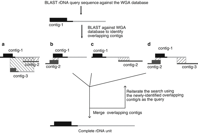
Flowchart of the strategy to construct the complete rDNA unit sequence. The rDNA query sequence is compared to the contigs obtained from the WGA to identify the primary rDNA -containing contig (contig-1). Contig-1 is then searched against the WGA database to identify additional rDNA -containing contigs. (a) If contig-1 has a complete rDNA unit, all other contigs will fully overlap it and nothing further needs to be done. (b–d) If the rDNA sequence is incomplete, iterations of identifying and merging overlapping contigs are performed until a complete rDNA unit is obtained. See text for more details
blastn -query <rdna_contig.fasta> -task blastn -db assembly.fasta -outfmt <number_to_define_output_format_type> -num_threads <number_of_threads>
Contigs that show matches to the rDNA query sequence are identified based on the BLAST e-value.
-
3.
Obtain the fasta sequences (from the assembly file assembly.fasta) and .ace files (from the “acedir” directory) of the matching contigs. Calculate the coverage using CLC Genomic workbench, and discard contigs that are <1 kb in length and/or have coverages similar to the unique region of the genome. The remaining contig(s) are potential rDNA -containing contigs. If more than one rDNA contig is identified, select the longest contig for further processing. If the second largest contig is slightly shorter than the largest contig (<1 kb) but has a higher read coverage, use this second contig instead.
-
4.
Open the .ace file for the rDNA contig in Consed. If the ends are of low coverage trim them by right clicking on the first base where low coverage region ends. Select the option “tear contig at this consensus position” and click “Do Tear.” This will open two new windows one for low coverage end contig and other has rest of the contig. Discard the low coverage contig and if needed trim the other end of the remaining contig. This trimmed contig is used for downstream analysis.
-
5.
To determine if the rDNA contig can be extended further, BLAST the contig sequence against the assembled contig BLAST database (Fig. 2). If the rDNA contig is incomplete, contigs overlapping with the query sequence will be identified. Discard contigs <1 kb in length and/or with read coverage similar to the unique region of the genome. Also discard contigs that fully overlap the query contig.
-
6.
Repeat this search iteratively using contigs that overlap both ends of the rDNA query sequence (when present) until only contig(s) hits with read coverages similar to that of the unique region of the genome are found. In our experience, usually only one or two iterations are required.
-
7.
Next, merge the identified contigs together to obtain the complete rDNA unit sequence. To achieve this, extract the .ace files for all the rDNA contigs identified. Then combine all the extracted .ace files into one .ace file. This has to be done manually: first, extract the first line of each .ace file and add the value of the fields representing the number of contigs and the number of reads in the file. Make a new header from this information in a new file that will contain information for all the rDNA contigs. For example, if three .ace files have to be concatenated and the values for their first lines are:
==> supercontig.ace.1 <==
AS 1 2797
==> supercontig.ace.2 <==
AS 1 138
==> supercontig.ace.3 <==
AS 3 11932
Then the first line of the new file combine.ace will be:
AS 5 14867
Next, remove the first line and copy the remaining data from each .ace file into the combine.ace file. This can be done using the following commands:
sed "/AS 1 2797/d" supercontig.ace.1 >> combine.ace
sed "/AS 1 138/d" supercontig.ace.2 >> combine.ace
sed "/AS 3 11932/d" supercontig.ace.3 >> combine.ace
-
8.
To merge the contigs, open the generated combine.ace file that contains all the overlapping rDNA contigs in Consed. Click the “Assembly View” button. This will open the “Assembly View” window followed by a popup “Which Contig to Show in Assembly View” window (if the popup window does not open automatically, go to “What to Show” and click on “In/exclude Contigs”). Increase the depth of coverage cut off value from 50 to an arbitrary value of 1000 to view contigs that have high read coverage, and click “Apply and Restart Assembly View.” This will regenerate the “Assembly View” window displaying all the contigs in the .ace file. Then go to “What to Show” and select “Sequence Matches.” This will open the “Which Sequence Matches to show in Assembly View” window that has different parameters for the aligner cross_match. Click the “run crossmatch” button to identify the overlapping regions between contigs (which are connected by vertical lines). To merge two contigs, double click the connecting line, opening the “Sequence Matches” window. Select the sequence in the window and click on “Show Alignment.” This will open the “Compare Contigs” window. If the second contig is a reverse complement in the “Sequence Matches” window, reverse complement the sequence by clicking the “complement just in this window” button in front of the contig name. Next, click the “Align” button to align the sequences and then click “Join Contigs.” This will merge the overlapping reads of both contigs and will generate a new longer merged contig. A new window will open that shows the consensus sequence of the generated contig together with all the reads. Save this new contig in the same .ace file (File → Save assembly). This will replace the contigs that were merged with the new one in the .ace file. Repeat until all overlapping contigs have been merged.
-
9.
By convention, the rDNA sequence is represented with the rRNA coding region transcribed from left to right first, followed by the IGS (Fig. 3a). To demarcate the rRNA coding region and the IGS in the merged rDNA contig, use BLAST with the closest available complete rRNA coding region sequence. Also by convention, the start of the rDNA unit is the transcriptional start site. Therefore, if the information is available, use BLAST to find the homologous transcriptional start site in the new rDNA sequence. Other annotations, such as promoters and terminators, can be added if possible.
Fig. 3 
Potential arrangements of the rRNA coding region and IGS in the merged rDNA contig. The position of the rRNA coding region (black boxes) and the IGS (grey lines) can vary in the merged rDNA contig. For example, (a) complete rRNA coding region followed by the IGS; (b) complete rDNA unit followed by a partial rDNA unit. The partial rDNA unit can have a complete rRNA coding region followed by a partial IGS (dotted grey line) or just a partial rRNA coding region; (c) partial rRNA coding regions on both ends of the contigs
-
10.
In some cases, the merged rDNA sequence has more than a single rDNA unit because of duplications at either end (Fig. 3b). Once the rRNA coding region has been identified, such instances are easy to rectify using BLAST to self-compare the merged rDNA sequence, whilst taking care not to remove regions that are actually repetitive within a single rDNA unit.
-
11.
In some cases the rDNA sequence has split the rRNA coding region across the ends of the contig (Fig. 3c). These contigs cannot be extended further, suggesting that the rRNA coding region is complete but segmented. In this case, remove the sequence of one of the partial rRNA coding regions and join it to the other end of the contig sequence such that the 5′-ETS/18S is either at the very start or end of the merged rDNA contig.
-
12.
If the merged rDNA contig has the rRNA coding region in the opposite orientation, make a reverse complement of the sequence to obtain the final rDNA unit sequence.
-
13.
In our experience, this approach is able to generate accurate and complete rDNA repeat sequences. However, to provide further confidence in the sequence obtained, it is possible to verify the rDNA repeat sequences using BAC clones containing rDNA if these are available (for example by screening whole genome BAC libraries). This is particularly desirable if the rDNA sequence contains repeats that are present elsewhere in the genome. There are two levels of verification: verifying the length of the repeat unit to demonstrate that a full-length rDNA sequence has been obtained (see Note 13 ); and verifying the sequence with NGS of rDNA -containing BAC clone(s) (see Note 14 ).


4 Notes
-
1.
To make this script work behind a network proxy, the following line in the original script:
my $res = LWP::UserAgent->new->request($req, sub { print $_[0] });
has to be modified to:
my $res = LWP::UserAgent->new();
$res->env_proxy();
$res->request($req, sub { print $_[0] });
-
2.
WGS data for an organism are sometimes generated as a joint project between two or more sequencing centers. In such cases, the data submitted by one sequencing center may only represent a fraction of the genome, and rDNA -containing contigs will likely be absent from the subsequent WGA. In that case, the assembly has to be performed again using a dataset from another sequencing center. To maximize the chances of using the best dataset, first individually map the data from all the sequencing centers that are involved in a given genome project to the rRNA coding region sequence of the species (or related species) using a Sanger read mapper (e.g., gsMapper). Then use the dataset from the sequencing center with the highest number of rDNA reads.
-
3.
The query_tracedb script command to download the TI number in binary format is:
query_tracedb "query page_size 40000 page_number N binary SPECIES_CODE=’PAN TROGLODYTES’ AND CENTER_NAME=’BI’ and TRACE_TYPE_CODE=’WGS’" > page_N.bin
where N is the page number.
-
4.
The command to download the fasta files is:
(echo -n "retrieve fasta 0b"; cat page_N.bin) | ./query_tracedb > data_N.fasta
(echo -n "retrieve quality 0b"; cat page_N.bin) | ./query_tracedb > data_N.qual
(echo -n "retrieve xml 0b"; cat page_N.bin) | ./query_tracedb > data_N.xml
where N is the page number.
-
5.
It is possible that because of sequencing depth or large genome size, a very large number of WGS reads are present for an organism from a project. Although it is recommended to take all the reads available reads to perform the WGA, it is possible to use just a subset of the WGS reads to speed up the assembly. If computational power is limited or the WGS read number is very high, divide the WGS data into two or three parts and perform WGAs for each of them. Then construct the rDNA sequence using each assembly and compare the rDNA sequences obtained. In theory, all the obtained rDNA sequences should be similar. The reduction of the input data can speed up the process, but it increases the chance that some of the rDNA is misassembled or missed during the assembly.
-
6.
Example of an NCBI entry’s fasta file header:
>gnl|ti|174190180 name:G591P603493FD5.T0 mate:174194532 CTAGNNNAAAGATCTGCCTGGGGGATTAGATCTAGCTGACAGTCAGGGTGGTGGTGGCC ……………………………………………………………………
-
7.
The following command:
sed -e "s/gnl|ti|[A-Za-z0-9]*\s//g" -e "s/mate:[A-Za-z0-9]*//g" -e "s/name://g" <input_fasta_file> >> fasta_file_with_modified_header.fasta
will change the header line to:
>G591P603493FD5.T0 CTAGNNNAAAGATCTGCCTGGGGGATTAGATCTAGCTGACAGTCAGGGTGGTGGTGGCC ……………………………………………………………………
-
8.
Example of an NCBI entry’s quality file header:
>gnl|ti|174190180 name:G591P603493FD5.T0 4 4 4 4 0 0 0 4 6 4 4 6 4 6 8 8 8 8 8 8 8 8 10 8 18 12 9 9 18 18 24 26 25 25 25 26 30 30 30 25 25 23 ……………………………………………………………………
-
9.
The field “type” in the traceinfo file is not part of the Trace archive format and hence its value has to be set in the configuration file reads_config.xml. The value of the type field can be “paired_production,” “unpaired_production,” or “transposon.” For Sanger WGS data, the value of the field “type” is usually “paired_production.” Further, sometimes the value of the field “insert_stdev” (standard deviation of the insert size in bp) is not defined, in which case 1/10th of the insert size can be used as the standard deviation.
-
10.
The command to modify the XML file to retain only the required information is:
grep -e "<trace>" -e "<trace_name>" -e "<plate_id>" -e "<well_id>" -e "<template_id>" -e "<clip_vector_left>" -e "<clip_vector_right>" -e "<insert_size>" -e "<insert_stdev>" -e "<trace_end>" -e "<center_name>" -e "<seq_lib_id>" -e "</trace>" <input_xml_file> >> xml:file_with_filtered_data.xml
Furthermore, Arachne requires an XML declaration as the first line of the file, and all the trace information has to be the child of the root element “trace_volume.” To fulfill both these requirements, the following two lines should be added at the start of the reads.xml file
<?xml version="1.0"?>
<trace_volume>
and the line below added as the very last line of the reads.xml file
</trace_volume>
-
11.
If the Arachne assembly breaks in the middle of a run, it can be restarted from the point it stopped with the following steps:
Step 1: Perform an Arachne run such that the all modules are run without generating any output using option NOGO = True:
/absolute/path/to/Assemblez PRE=/path/to/working/directory DATA=data RUN=run num_cpus=number_of_cpu num_cpus_pi=10 ACE=True REMOVE_INTERMEDIATES=False NOGO=True > log.txt
The obtained file log.txt will have the commands for each step that has to be run during the assembly.
Step 2: The “RUN” directory also has a log file assemblez.log that has details of all the commands used during the assembly. Search assemblez.log for the last generated output directory:
grep "OUTDIR" /path/to/run/assemblez.log | tail –n 1
Step 3: Search the module that has generated the last output directory in the log.txt file from Step 1:
grep "<name of last output directory >" log.txt
Step 4: Restart the assembly from the module at which Arachne was broken using the command:
/absolute/path/to/Assemblez PRE=/path/to/working/directory DATA=data RUN=run num_cpus=number_of_cpu num_cpus_pi=10 ACE=True REMOVE_INTERMEDIATES=False START=<Module_name>
where “Module_name” is the module that generated the last output directory.
-
12.
The ACE file format stores the contig information. This file format was initially developed for the visualization and manipulation of contigs using Consed, but was later adopted by other Sanger sequence assemblers . A single .ace file can contain information for more than one contig. The first line of an .ace file shows the number of contigs and total number reads in the file, and subsequent lines have information about the individual contigs. The details of the ACE file format are described in the Consed manual [84].
-
13.
BAC clones, with an average insert size of ~175 kb, are expected to contain at least 4–5 rDNA copies, as the rDNA is up to ~45 kb in length [26, 27]. I-PpoI, a homing enzyme, cuts only at one site in the rDNA repeat (in the 18S rRNA coding region), allowing liberation of single rDNA units from a BAC clone. Therefore, the length of BAC rDNA repeat units can be estimated by gel electrophoresis following I-PpoI digestion. If the rDNA unit length is small (up to ~15 kb), conventional gel electrophoresis using low percent agarose gels can be used to determine the length. However, for larger rDNA units pulsed field gel electrophoretic separations are necessary. We found that Field Inversion Gel Electrophoresis (FIGE) implemented on a CHEF electrophoresis apparatus can accurately determine long rDNA unit lengths. We have found that FIGE gels seem to consistently overestimate the rDNA unit length by ~1 kb. The rDNA unit band can be confirmed by Southern hybridization using an rRNA coding region probe if necessary.
-
14.
A WGA rDNA sequence can be further verified by mapping NGS reads from rDNA -containing BAC clones to the WGA rDNA sequence. This allows detection of relatively small-scale errors in the rDNA sequence. In our experience, some parts of the rRNA coding region are highly biased against in Illumina sequencing outputs, as discussed earlier. Thus reads from these regions can be absent from the sequencing data for the rDNA BAC clones. When WGA and BAC rDNA sequences are compared, these regions appear as gaps in the BAC rDNA sequences. These gaps should not be interpreted as misassemblies in the WGA rDNA sequences, but as sequencing limitations. Because the rRNA coding regions are well characterized in most eukaryotic lineages, such cases are straightforward to diagnose.
References
Yue F, Cheng Y, Breschi A et al (2014) A comparative encyclopedia of DNA elements in the mouse genome. Nature 515:355–364
Encode Project Consortium (2012) An integrated encyclopedia of DNA elements in the human genome. Nature 489:57–74
Koch CM, Andrews RM, Flicek P et al (2007) The landscape of histone modifications across 1% of the human genome in five human cell lines. Genome Res 17:691–707
Pei B, Sisu C, Frankish A et al (2012) The GENCODE pseudogene resource. Genome Biol 13:R51
Orom UA, Derrien T, Beringer M et al (2010) Long noncoding RNAs with enhancer-like function in human cells. Cell 143:46–58
Djebali S, Davis CA, Merkel A et al (2012) Landscape of transcription in human cells. Nature 489:101–108
Nam JW, Bartel DP (2012) Long noncoding RNAs in C. elegans. Genome Res 22:2529–2540
Brown JB, Boley N, Eisman R et al (2014) Diversity and dynamics of the Drosophila transcriptome. Nature 512:393–399
Gerstein MB, Rozowsky J, Yan KK et al (2014) Comparative analysis of the transcriptome across distant species. Nature 512:445–448
Scally A, Dutheil JY, Hillier LW et al (2012) Insights into hominid evolution from the gorilla genome sequence. Nature 483:169–175
The Chimpanzee Sequencing and Analysis Consortium (2005) Initial sequence of the chimpanzee genome and comparison with the human genome. Nature 437:69–87
International Chicken Genome Sequencing Consortium (2004) Sequence and comparative analysis of the chicken genome provide unique perspectives on vertebrate evolution. Nature 432:695–716
Naumova N, Imakaev M, Fudenberg G et al (2013) Organization of the mitotic chromosome. Science 342:948–953
Ho JW, Jung YL, Liu T et al (2014) Comparative analysis of metazoan chromatin organization. Nature 512:449–452
Rao SS, Huntley MH, Durand NC et al (2014) A 3D map of the human genome at kilobase resolution reveals principles of chromatin looping. Cell 159:1665–1680
Eichler EE, Clark RA, She X (2004) An assessment of the sequence gaps: unfinished business in a finished human genome. Nat Rev Genet 5:345–354
Floutsakou I, Agrawal S, Nguyen TT et al (2013) The shared genomic architecture of human nucleolar organizer regions. Genome Res 23:2003–2012
Leem SH, Kouprina N, Grimwood J et al (2004) Closing the gaps on human chromosome 19 revealed genes with a high density of repetitive tandemly arrayed elements. Genome Res 14:239–246
Dunham A, Matthews LH, Burton J et al (2004) The DNA sequence and analysis of human chromosome 13. Nature 428:522–528
Zody MC, Garber M, Sharpe T et al (2006) Analysis of the DNA sequence and duplication history of human chromosome 15. Nature 440:671–675
Hattori M, Fujiyama A, Taylor TD et al (2000) The DNA sequence of human chromosome 21. Nature 405:311–319
Heilig R, Eckenberg R, Petit JL et al (2003) The DNA sequence and analysis of human chromosome 14. Nature 421:601–607
McClintock B (1934) The relation of a particular chromosomal element to the development of the nucleoli in Zea mays. Z Zellforsch Mikrosk Anat 21:294–326
Ritossa FM, Spiegelman S (1965) Localization of DNA complementary to ribosomal RNA in the nucleolus organizer region of Drosophila melanogaster. Proc Natl Acad Sci U S A 53:737–745
Phillips RL, Kleese R, Wang SS (1971) The nucleolus organizer region of maize (Zea mays L.): chromosomal site of DNA complementary to ribosomal RNA. Chromosoma 36:79–88
Thiry M, Lafontaine DL (2005) Birth of a nucleolus: the evolution of nucleolar compartments. Trends Cell Biol 15:194–199
Grozdanov P, Georgiev O, Karagyozov L (2003) Complete sequence of the 45-kb mouse ribosomal DNA repeat: analysis of the intergenic spacer. Genomics 82:637–643
van Keulen H, Gutell RR, Campbell SR et al (1992) The nucleotide sequence of the entire ribosomal DNA operon and the structure of the large subunit rRNA of Giardia muris. J Mol Evol 35:318–328
Spear BB (1980) Isolation and mapping of the rRNA genes in the macronucleus of Oxytricha fallax. Chromosoma 77:193–202
Birnstiel ML, Chipchase MI, Hyde BB (1963) The nucleolus, a source of ribosomes. Biochim Biophys Acta 76:454–462
Kobayashi T, Ganley AR (2005) Recombination regulation by transcription-induced cohesin dissociation in rDNA repeats. Science 309:1581–1584
Donati G, Montanaro L, Derenzini M (2012) Ribosome biogenesis and control of cell proliferation: p53 is not alone. Cancer Res 72:1602–1607
Derenzini M, Montanaro L, Chilla A et al (2005) Key role of the achievement of an appropriate ribosomal RNA complement for G1-S phase transition in H4-II-E-C3 rat hepatoma cells. J Cell Physiol 202:483–491
Deisenroth C, Zhang Y (2010) Ribosome biogenesis surveillance: probing the ribosomal protein-Mdm2-p53 pathway. Oncogene 29:4253–4260
Audas TE, Jacob MD, Lee S (2012) Immobilization of proteins in the nucleolus by ribosomal intergenic spacer noncoding RNA. Mol Cell 45:147–157
Zhang LF, Huynh KD, Lee JT (2007) Perinucleolar targeting of the inactive X during S phase: evidence for a role in the maintenance of silencing. Cell 129:693–706
Clos J, Normann A, Ohrlein A et al (1986) The core promoter of mouse rDNA consists of two functionally distinct domains. Nucleic Acids Res 14:7581–7595
Doelling JH, Gaudino RJ, Pikaard CS (1993) Functional analysis of Arabidopsis thaliana rRNA gene and spacer promoters in vivo and by transient expression. Proc Natl Acad Sci U S A 90:7528–7532
Haltiner MM, Smale ST, Tjian R (1986) Two distinct promoter elements in the human rRNA gene identified by linker scanning mutagenesis. Mol Cell Biol 6:227–235
Pfleiderer C, Smid A, Bartsch I et al (1990) An undecamer DNA sequence directs termination of human ribosomal gene transcription. Nucleic Acids Res 18:4727–4736
Grummt I, Maier U, Ohrlein A et al (1985) Transcription of mouse rDNA terminates downstream of the 3′ end of 28S RNA and involves interaction of factors with repeated sequences in the 3′ spacer. Cell 43:801–810
Nemeth A, Perez-Fernandez J, Merkl P et al (2013) RNA polymerase I termination: where is the end? Biochim Biophys Acta 1829:306–317
Pape LK, Windle JJ, Mougey E et al (1989) The Xenopus ribosomal DNA 60-and 81-base-pair repeats are position-dependent enhancers that function at the establishment of the preinitiation complex: analysis in vivo and in an enhancer-responsive in vitro system. Mol Cell Biol 9:5093–5104
Little RD, Platt TH, Schildkraut CL (1993) Initiation and termination of DNA replication in human rRNA genes. Mol Cell Biol 13:6600–6613
Yoon Y, Sanchez JA, Brun C et al (1995) Mapping of replication initiation sites in human ribosomal DNA by nascent-strand abundance analysis. Mol Cell Biol 15:2482–2489
Gencheva M, Anachkova B, Russev G (1996) Mapping the sites of initiation of DNA replication in rat and human rRNA genes. J Biol Chem 271:2608–2614
Yu GL, Blackburn EH (1990) Amplification of tandemly repeated origin control sequences confers a replication advantage on rDNA replicons in Tetrahymena thermophila. Mol Cell Biol 10:2070–2080
Daniel DC, Johnson EM (1989) Selective initiation of replication at origin sequences of the rDNA molecule of Physarum polycephalum using synchronous plasmodial extracts. Nucleic Acids Res 17:8343–8362
Van’t Hof J, Hernandez P, Bjerknes CA et al (1987) Location of the replication origin in the 9-kb repeat size class of rDNA in pea (Pisum sativum). Plant Mol Biol 9:87–95
Botchan PM, Dayton AI (1982) A specific replication origin in the chromosomal rDNA of Lytechinus variegatus. Nature 299:453–456
Gogel E, Langst G, Grummt I et al (1996) Mapping of replication initiation sites in the mouse ribosomal gene cluster. Chromosoma 104:511–518
Muller M, Lucchini R, Sogo JM (2000) Replication of yeast rDNA initiates downstream of transcriptionally active genes. Mol Cell 5:767–777
Coffman FD, He M, Diaz M-L et al (2006) Multiple initiation sites within the human ribosomal RNA gene. Cell Cycle 5:1223–1233
Coffman FD, Georgoff I, Fresa KL et al (1993) In vitro replication of plasmids containing human ribosomal gene sequences: origin localization and dependence on an aprotinin-binding cytosolic protein. Exp Cell Res 209:123–132
Akamatsu Y, Kobayashi T (2015) The human RNA polymerase I transcription terminator complex acts as a replication fork barrier that coordinates the progress of replication with rRNA transcription activity. Mol Cell Biol 35:1871–1881
Dimitrova DS (2011) DNA replication initiation patterns and spatial dynamics of the human ribosomal RNA gene loci. J Cell Sci 124:2743–2752
Brewer BJ, Fangman WL (1988) A replication fork barrier at the 3′ end of yeast ribosomal RNA genes. Cell 56:637–643
Lopez-estrano C, Schvartzman JB, Krimer DB et al (1998) Co-localization of polar replication fork barriers and rRNA transcription terminators in mouse rDNA. J Mol Biol 277:249–256
Lopez-Estrano C, Schvartzman JB, Krimer DB et al (1999) Characterization of the pea rDNA replication fork barrier: putative cis-acting and trans-acting factors. Plant Mol Biol 40:99–110
Wiesendanger B, Lucchini R, Koller T et al (1994) Replication fork barriers in the Xenopus rDNA. Nucleic Acids Res 22:5038–5046
Grandori C, Gomez-Roman N, Felton-Edkins ZA et al (2005) c-Myc binds to human ribosomal DNA and stimulates transcription of rRNA genes by RNA polymerase I. Nat Cell Biol 7:311–318
Kern SE, Kinzler KW, Bruskin A et al (1991) Identification of p53 as a sequence-specific DNA-binding protein. Science 252:1708–1711
Jacob MD, Audas TE, Mullineux ST et al (2012) Where no RNA polymerase has gone before: novel functional transcripts derived from the ribosomal intergenic spacer. Nucleus 3:315–319
Bierhoff H, Schmitz K, Maass F et al (2010) Noncoding transcripts in sense and antisense orientation regulate the epigenetic state of ribosomal RNA genes. Cold Spring Harb Symp Quant Biol 75:357–364
Mayer C, Neubert M, Grummt I (2008) The structure of NoRC-associated RNA is crucial for targeting the chromatin remodelling complex NoRC to the nucleolus. EMBO Rep 9:774–780
Mayer C, Schmitz KM, Li J et al (2006) Intergenic transcripts regulate the epigenetic state of rRNA genes. Mol Cell 22:351–361
Saka K, Ide S, Ganley AR et al (2013) Cellular senescence in yeast is regulated by rDNA noncoding transcription. Curr Biol 23:1794–1798
Prokopowich CD, Gregory TR, Crease TJ (2003) The correlation between rDNA copy number and genome size in eukaryotes. Genome 46:48–50
Long EO, Dawid IB (1980) Repeated genes in eukaryotes. Annu Rev Biochem 49:727–764
Stage DE, Eickbush TH (2007) Sequence variation within the rRNA gene loci of 12 Drosophila species. Genome Res 17:1888–1897
Ganley AR, Kobayashi T (2007) Highly efficient concerted evolution in the ribosomal DNA repeats: total rDNA repeat variation revealed by whole-genome shotgun sequence data. Genome Res 17:184–191
James SA, O’Kelly MJ, Carter DM et al (2009) Repetitive sequence variation and dynamics in the ribosomal DNA array of Saccharomyces cerevisiae as revealed by whole-genome resequencing. Genome Res 19:626–635
Gonzalez IL, Sylvester JE (1995) Complete sequence of the 43-kb human ribosomal DNA repeat: analysis of the intergenic spacer. Genomics 27:320–328
Li Z, Chen Y, Mu D et al (2012) Comparison of the two major classes of assembly algorithms: overlap-layout-consensus and de-bruijn-graph. Brief Funct Genomics 11:25–37
Flicek P, Birney E (2009) Sense from sequence reads: methods for alignment and assembly. Nat Methods 6:S6–S12
Margulies M, Egholm M, Altman WE et al (2005) Genome sequencing in microfabricated high-density picolitre reactors. Nature 437:376–380
Myers EW, Sutton GG, Delcher AL et al (2000) A whole-genome assembly of Drosophila. Science 287:2196–2204
Green P. Documentation for phrap and cross_match. http://www.phrap.org/phredphrap/phrap.html. Accessed 21 August 2015
Chevreux B, Wetter T, Suhai S (1999) Genome sequence assembly using trace signals and additional sequence information. In: German Conference on Bioinformatics, pp 45–56
Jaffe DB, Butler J, Gnerre S et al (2003) Whole-genome sequence assembly for mammalian genomes: Arachne 2. Genome Res 13:91–96
Batzoglou S, Jaffe DB, Stanley K et al (2002) ARACHNE: a whole-genome shotgun assembler. Genome Res 12:177–189
Burton J (2008) Repeat. https://www.broadinstitute.org/crd/wiki/index.php/Repeat. Accessed 26 August 2015
Gordon D, Abajian C, Green P (1998) Consed: a graphical tool for sequence finishing. Genome Res 8:195–202
Gordon D (2015) Consed 29.0 Documentation. http://www.phrap.org/consed/distributions/README.29.0.txt. Accessed 26 August 2015
Searching Tips. NCBI. http://www.ncbi.nlm.nih.gov/Traces/trace.cgi?view=search_tips. Accessed 26 August 2015
Heiman D, Burton J (2007) XML ancillary files. https://www.broadinstitute.org/crd/wiki/index.php/XML_ancillary_files. Accessed 26 August 2015
Burton J, Gnerre S (2006) Directory tree. http://www.broadinstitute.org/crd/wiki/index.php/Directory_tree. Accessed 26 August 2015
Heiman D, Burton J, Grabherr MG (2006) Input. http://www.broadinstitute.org/crd/wiki/index.php/Input. Accessed 26 August 2015
Heiman D, Burton J (2007) Reads config.xml. http://www.broadinstitute.org/crd/wiki/index.php/Reads_config.xml. Accessed 26 August 2015
Burton J (2008) FindXmlFeatures. http://www.broadinstitute.org/crd/wiki/index.php/FindXmlFeatures. Accessed 26 August 2015
Burton J, Gnerre S, Grabherr MG (2006) Output. https://www.broadinstitute.org/crd/wiki/index.php/Output. Accessed 26 August 2015
Author information
Authors and Affiliations
Corresponding authors
Editor information
Editors and Affiliations
Rights and permissions
Copyright information
© 2016 Springer Science+Business Media New York
About this protocol
Cite this protocol
Agrawal, S., Ganley, A.R.D. (2016). Complete Sequence Construction of the Highly Repetitive Ribosomal RNA Gene Repeats in Eukaryotes Using Whole Genome Sequence Data. In: Németh, A. (eds) The Nucleolus. Methods in Molecular Biology, vol 1455. Humana Press, New York, NY. https://doi.org/10.1007/978-1-4939-3792-9_13
Download citation
DOI: https://doi.org/10.1007/978-1-4939-3792-9_13
Published:
Publisher Name: Humana Press, New York, NY
Print ISBN: 978-1-4939-3790-5
Online ISBN: 978-1-4939-3792-9
eBook Packages: Springer Protocols