
Abstract
The analysis of protein half-life and degradation dynamics has proven critically important to our understanding of a broad and diverse set of biological conditions ranging from cancer to neurodegeneration. Historically these protein turnover measures have been performed in cells by monitoring protein levels after “pulse” labeling of newly synthesized proteins and subsequent chase periods. Comparing the level of labeled protein remaining as a function of time to the initial level reveals the protein’s half-life. In this method we provide a detailed description of the workflow required for the determination of protein turnover rates on a whole proteome scale in vivo.
Our approach starts with the metabolic labeling of whole rodents by restricting all the nitrogen in their diet to exclusively nitrogen-15 in the form of spirulina algae. After near complete organismal labeling with nitrogen-15, the rodents are then switched to a normal nitrogen-14 rich diet for time periods of days to years. Tissues are harvested, the extracts are fractionated, and the proteins are digested to peptides. Peptides are separated by multidimensional liquid chromatography and analyzed by high resolution orbitrap mass spectrometry (MS). The nitrogen-15 containing proteins are then identified and measured by the bioinformatic proteome analysis tools Sequest, DTASelect2, and Census. In this way, our metabolic pulse-chase approach reveals in vivo protein decay rates proteome-wide.
Access provided by CONRICYT – Journals CONACYT. Download protocol PDF
Key words
- Proteomics
- Mass spectrometry
- Protein half-life
- Protein decay dynamics
- Stable isotope labeling of mammals
- Nitrogen-15
- SILAC
- SILAM
- Extremely long-lived proteins
1 Introduction
To determine the rate of protein decay, new and old versions of each protein must be discernable and ideally both be measurable. Typically cells are initially “pulsed” with a traceable molecular label (such as methionine enriched with sulfur-35 atoms) which are incorporated into newly synthesized proteins and subsequently “chased” with a normal containing methionine (sulfur-32 fraction of 95.02 %) [1, 2]. By comparing the initial amount of a specific labeled protein to that remaining as a function of time, a measure of protein half-life can be obtained [3]. These analyses can also provide key information on the possibility that different pools of the same protein exist and have dissimilar decay kinetics. Recently, proteomic technologies have been applied to gain insight into the analysis of protein turnover dynamics on a proteome-wide scale. By combining the yeast whole genome tap-tag gene library, translation inhibition with cycloheximide, and epitope tag western blot analysis, it was determined that on average the lifetime of a yeast protein is about 43 min [4]. In cultured HeLa and C2C12 cells, “pulse-only” stable isotope labeling of cells in culture (SILAC) for several durations with time course mass spectrometry (MS) analysis showed average protein half-life in mouse and human cells <2 days [5]. In mice, by using MS analysis to measure the rate by which isotopes are metabolically incorporated into proteins and modeling it has been suggested that on average proteins in brain tissue have a lifetime of 9.0 days, liver 3.0 days, and blood 3.5 days [6, 7].
We have developed a straightforward systematic approach to monitor protein decay dynamics on a global scale in the most relevant biological context, in vivo. Our approach has verified previously reported rapid degradation dynamics for nearly all proteins. Unexpectedly we also find a limited number of intracellular extremely long-lived proteins (ELLPs) which reside in the nucleus and cytoplasm of postmitotic neurons [8, 9]. Our approach also confirmed the existence ELLPs in the myelin sheath and eye lens [10–12]. The application of our approach to proteinopathy disease mouse models (such as Alzheimer’s, Parkinson’s, and Huntington’s disease) could provide new insight into pathogenic mechanisms by identifying disease-specific long-lived proteins.
2 Materials
Buffers and solutions for MS analysis should be prepared with analytical chromatography grade solvents, and for biochemical experiments we prepared buffers with ultra-pure water (Milli-Q® Water Purification Systems, 18-megohm-cm deionized water). Solutions should be stored at room temperature unless otherwise indicated. To minimize keratin contamination gloves should be worn during the preparation of all buffers and samples.
2.1 Nitrogen-15 or Nitrogen-14 Spirulina Rodent Chow
-
1.
Nitrogen-15 enriched spirulina algae: Nitrogen-15 enriched (>94 %) spirulina were purchased from Cambridge Isotopes [13], Cambridge, MA, USA, or can be grown and prepared in-house as previously described [14–16].
-
2.
Rodent chow: Rodent chow has been prepared by mixing nitrogen-15 or nitrogen-14 spirulina with protein-free diet mixture powder (Harlan TD 93328) in a 1 to 3 ratio. Pellets were prepared by adding ultra-pure water to the power mixture and working the mixture into dough shaped into cylinders. Individual ~2-cm discs we cut from the cylinders and dried at 60 °C for 2–4 h and then at 35 °C overnight on screen trays in an Excalibur food dehydrator [17]. Alternatively, nitrogen-15 spirulina containing chow can be purchased pre-prepared from CIL/Harlan Laboratories Inc. with 22 % protein/65 % carbohydrate (carbon, hydrogen, oxygen as CHO), 13 % fat composition (see Note 1 ).
2.2 Representative Protein Fractionation
-
1.
Tissue homogenization buffer: 0.32 M sucrose , 4 mM Hepes (pH 7.4), 1 mM MgCl2, and protease inhibitors (Sigma) (see Note 2 ). 1 M Hepes, add 600 mL water to a glass beaker, weigh and add 238.3 g of Hepes, add stir bar to dissolve on a stir plate. Determine pH and adjust with HCl or NaOH to pH 7.4 final. Transfer to a graduated cylinder and add water to 1 L. Store at 4 °C. 1 M MgCl2, add 500 mL water to a glass beaker, weigh and add 203.3 g of MgCl2 6H2O, add stir bar to dissolve on a stir plate. Transfer to a graduated cylinder and add water to 1 L. To a 250 mL glass beaker, a stir bar, add 50 mL of water, 5 mL of 1 M Hepes (pH 7.4), 0.1 mL of 1 M MgCl2, and 10.9 g of Sucrose. Transfer to a 100 mL graduated cylinder and add water to 100 mL [18].
-
2.
Sucrose gradient buffers (0.85 M/1.0 M/1.2 M/2.0 M): Weigh 28.9, 34.0, 40.9, 69.1 g and prepare 100 mL of buffer as described above except substitute the indicated amount of sucrose for each buffer.
-
3.
2,2,2-Trichloroacetic acid (TCA) buffer: prepare a 100 % (wt/vol) TCA solution with water.
2.3 Protein Digestion
-
1.
Urea protein denaturation buffer : Dissolve 0.395 g of solid Ammonium bicarbonate (AMBC) in 100 mL of water to prepare 50 mM adjust to pH 7.5 as described above; aliquot and store at −20 °C. Add 0.240 g of urea to 320 μl of AMBC buffer to prepare 8 M solution (see Note 3 ).
-
2.
ProteaseMAX surfactant buffer: Dissolve solid ProteaseMAX in 500 μl of AMBC to prepare 0.2 % solution or 100 μl for 1 % (see Note 4 ).
-
3.
Reduction buffer: Dissolve solid Tris (2-carboxyethyl) phosphine hydrochloride (TCEP) in AMBC to prepare 0.5 M solution (see Note 5 ).
-
4.
Alkylation buffer: Dissolve solid Iodoacetamide in AMBC and prepare 1 M solution.
-
5.
Trypsin buffer: Dissolve 20 μg vial of lyophilized trypsin (Promega) in 40 μl of buffer (see Note 6 ).
2.4 Liquid Chromatography
-
1.
HPLC buffer A: 95 % water, 5 % acetonitrile, and 0.1 % formic acid (vol/vol).
-
2.
HPLC buffer B: 20 % water, 80 % acetonitrile, and 0.1 % formic acid (vol/vol).
-
3.
HPLC buffer C: 500 mM ammonium acetate, 5 % (vol/vol) acetonitrile, and 0.1 % (vol/vol) formic acid.
-
4.
Make Kasil frit and prepare multidimensional protein identification (MudPIT) column by bomb packing strong cation exchange (SCX )/reversed phase resins as previously described [19–21].
2.5 Mass Spectrometer
-
1.
Tune and calibrate electrospray high resolution orbitrap mass spectrometer (Thermo Scientific™ Orbitrap Velos Pro or Orbitrap Tribrid Fusion) per the manufacturer’s instructions with Pierce LTQ Velos ESI Positive Ion Calibration Solution (see Note 7 ).
2.6 Proteomic Analysis Software
-
1.
IP2 (Integrated Proteomic Analysis environment is commercially available; http://integratedproteomics.com/).
-
2.
RawExtractor (Spectra extraction tool is freely downloadable; http://fields.scripps.edu/researchtools.php).
-
3.
Sequest/Prolucid (Protein database search algorithm is freely downloadable; http://fields.scripps.edu/researchtools.php).
-
4.
DTASelect2 (protein dataset filtering tool is freely downloadable; http://fields.scripps.edu/researchtools.php).
-
5.
Census (protein quantitation software is freely downloadable; http://fields.scripps.edu/researchtools.php).
3 Methods
Perform all procedures at room temperature unless noted.
3.1 Metabolic Labeling of Whole Rodents
-
1.
Obtain two recently weaned female rats and allow acclimating in the university approved animal facility for several days (see Note 8 ).
-
2.
Replace standard rodent chow with nitrogen-15 containing spirulina chow and house for >10 weeks (see Note 9 ).
-
3.
Introduce male breeder rat into breeding cages and monitor female rat for weight gain indicative of successful pregnancy (see Note 10 ).
-
4.
Closely monitor cages for pups and document successful breeding. Continue feeding with exclusively nitrogen-15 containing spirulina chow while pups are nursing (see Note 11 ).
-
5.
Once pups are weaned, feed with exclusively nitrogen-15 containing spirulina chow for additional 3–4 weeks.
-
6.
Start chase period by switching to regular nitrogen-14 rodent chow (see Note 12 ).
3.2 Tissue Harvest
-
1.
Sacrifice time = 0 animal with CO2 as the primary mechanism and secondarily by decapitation.
-
2.
Harvest all tissues with standard dissection procedures and carefully label and freeze each tissue in a separate tube in liquid nitrogen and then store at −80 °C.
-
3.
Sacrifice littermates at additional time points and repeat dissection and tissue harvesting as needed (see Note 13 ) (Fig. 1).
Fig. 1 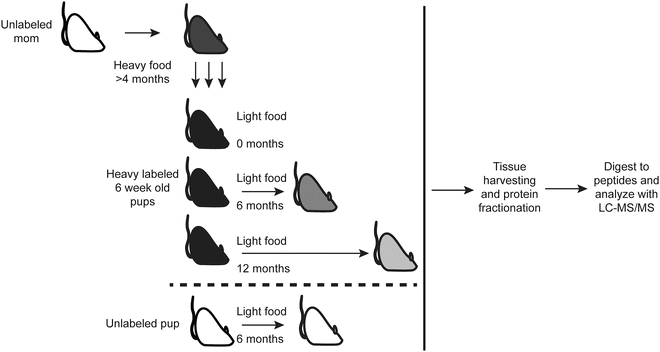
Metabolic pulse chase labeling of rats workflow to measure protein turnover dynamics in vivo. Freshly weaned female rat (first generation) is obtained and the diet is switched completely to nitrogen-15 containing food for 10–16 weeks. Male rat is introduced and female rat remains on nitrogen-15 diet while pregnant and during the nursing of her pups. Pups (second generation) are sacrificed at several time points including time = 0, before switching to nitrogen-14 chow. For the identification and analysis of extremely long-lived proteins, we found 6 month and 12 month reliable chase durations. As a negative control, we analyze an unlabeled pup after feeding regular nitrogen-14 chow. After the animals are sacrificed, their tissues are dissected, proteins solubilized and then fractionated. The proteins are then digested to peptides prior to LC-MS and bioinformatic analysis

3.3 Representative Protein Fractionation from Brain Tissue
-
1.
Homogenize rat brain in 12 mL of tissue homogenization buffer on ice and centrifuge at 4 °C, 1500 × g for 15 min, and the supernatant was collected (postnuclear supernatant).
-
2.
Centrifuge supernatant at 4 °C, 18,000 × g for 20 min, collect the resulting supernatant (cytosol) and pellet (crude membrane).
-
3.
Resuspend pellet in homogenization buffer and load it onto a 0.85 M/1.0 M/1.2 M sucrose gradient and centrifuge at 4 °C, 78,000 × g for 120 min, and collect the material focused at the 1.0 M/1.2 M interface (synaptosomes).
-
4.
Add Triton X-100 to 0.5 % final concentration and extract at 4 °C, by end-over-end agitation for 20 min.
-
5.
Centrifuge the extract at 4 °C, 32,000 × g for 20 min, and collect the supernatant (soluble synaptosome).
-
6.
Resuspend pellet in homogenization buffer and load onto a 1.0 M/1.5 M/2.0 M sucrose gradient and centrifuge at 4 °C, 170,000 × g for 120 min [18].
-
7.
Collected material at the 1.5 M/2.0 M interface (postsynaptic density, PSD).
-
8.
Add 0.5 % Triton X-100 and detergent soluble material extracted at 4 °C, by end-over-end agitation for 10 min.
-
9.
Centrifuge extract at 4 °C, 100,000 × g for 20 min, and resuspend the pellet in homogenization buffer (purified PSD) .
3.4 Protein Digestion and Peptide Preparation
-
1.
To each fraction (100 μg) add TCA to 20 % (vol/vol) final concentration, vortex, incubate on ice at 4 °C for 4 h to overnight (see Note 14 ).
-
2.
Centrifuge at 14,000 × g for 45 min at 4 °C.
-
3.
Discard supernatant and wash the pellet with 1 mL of ice-cold acetone.
-
4.
Centrifuge the tube at 14,000 × g for 10 min at 4 °C.
-
5.
Remove the acetone and wash the pellet with 1 mL of ice-cold acetone (two washes in total).
-
6.
Centrifuge the tube at 14,000 × g for 10 min at 4 °C.
-
7.
Remove supernatant and air-dry the pellet at room temperature.
-
8.
Add 50 μl of urea buffer and resuspend dry protein pellet and vortex for at least 1 h.
-
9.
Add 50 μl of 0.2 % (wt/vol) ProteaseMAX and vortex for at least 1 h.
-
10.
Add 1 μl of TCEP buffer and vortex the mixture for at least 1 additional hour.
-
11.
Add 2 μl of IAA buffer, mix well, and incubate in the dark for 20 min.
-
12.
Squelch alkylation reaction by adding 5 μl of TCEP buffer.
-
13.
Add 150 μl of AMBC and mix well (see Note 15 ).
-
14.
Add 2.5 μl of 1 % (wt/vol) proteaseMAX and briefly vortex.
-
15.
Add 2–4 μg of sequencing-grade trypsin and incubate the mixture overnight at 37 °C with shaking.
-
16.
Recover the samples and store them at −80 °C (see Note 16 ).
3.5 Loading the Peptides on the Column
-
1.
Thaw peptides and acidify to a 5 % (vol/vol) final concentration with formic acid.
-
2.
Centrifuge the tube at 14,000 × g for 15 min at room temperature and transfer supernatant to a new tube.
-
3.
Directly Load peptide sample onto SCX /RP column with a bomb at a pressure of 500–1000 psi [22] (see Note 17 ).
-
4.
Wash column with buffer A for 30 min on bomb.
-
5.
Pull a 15-cm tip of 100-μm glass capillary and use bomb to pack RP resin.
-
6.
Flow buffer B for 15 min to wash the analytical tip.
-
7.
Flow buffer A for 15 min to equilibrate the analytical tip.
3.6 Liquid Chromatography/Mass Spectrometry
-
1.
Connect the MudPIT column (frit connected to the analytical tip with an IDEX union) to the HPLC pump and start buffer A to ensure stable flow rates and pressure without leaks.
-
2.
Generate 11-step LC and MS methods with Xcalibur software.
-
3.
Start the 11-step LC/MS sequence with the Xcalibur software on the MS computer (see Note 18 ). The analysis will be performed over a 22–24 h time period per sample analysis.
3.7 Bioinformatic Data Analysis
-
1.
Process acquired .RAW files by first extracting them to .MS1 and .MS2 format with RawExtractor software on the mass spectrometer’s PC [23].
-
2.
Upload all files (33 total, 11 .RAW, 11 .MS1, and 11 .MS2) into the IP2 software.
-
3.
Perform Prolucid heavy and light database search with the rat (species matched) protein database and parameters such as a fixed modification of 57.02146 on cysteine, possessing at least one tryptic terminus, and with unlimited missed cleavages [24] (see Note 19 ) (Fig. 2).
Fig. 2 
Bioinformatic spectral analysis paradigm. Theoretical representation of a zoomed MS1 spectral scan, starred peaks are selected for MS2 and indicate identification of both the abundant nitrogen-14 light (starred peak) and the low abundance nitrogen-15 heavy (starred peak) isotopic peaks. MS1 ion abundance is analyzed as reconstructed chromatograms based on the identification of the light or heavy peak (grey bar). To determine the peptide abundances, the area under each curve is calculated and compared to determine the relative abundances of the light “new” and heavy “old” peptides
-
4.
Filter and control false-discovery rate for each dataset individually with DTASelect with target-decoy strategy (concatenated forward-reverse amino acid sequence protein database) to ensure a 0–1 % false discovery rate at the protein level [25].
-
5.
To view the proteins which are identified (based on matched MS scan) only in the heavy search, run “heavy only” DTASelect analysis.
-
6.
Perform peptide quantitation and enrichment analysis with Census software within IP2 [26–28] (see Note 20 ) (Fig. 3).
Fig. 3 
Incorporation of MS1 isotopic envelope shape measurement into protein turnover analysis workflow increases confidence and shows system-wide protein degradation dynamics. (a) Theoretical MS1 isotopic spectral envelope after 0 or 30 day nitrogen-14 chase periods, both showing identification of the fully heavy labeled peptide species (100 % of nitrogen atoms are nitrogen-15). The corresponding “light” isotopic envelope enrichment is determined by comparing the acquired m/z isotopic envelope shape to a broad range of predicted enrichment peak patterns to determine the percentage of nitrogen-15 atoms. (b) Binned peptide nitrogen-15 enrichment distribution from synaptosome extracts after 0, 2, 7, 30, or 180 days of nitrogen-14 chase


4 Notes
-
1.
Spirulina algae have been successfully grown on nitrogen-15 salts in research labs or can be purchased commercially [7, 29]. We have found it to be most efficient to purchase the nitrogen-15 spirulina already prepared as ready to eat chow.
-
2.
We present here a representative protein fractionation scheme to enrich for postsynaptic density proteins. Any protein fractionation or enrichment procedure (that is compatible with MS analysis) could be utilized for the investigation of protein turnover dynamics depending on the protein’s specific localization characteristics.
-
3.
We find that 50 mM AMBC is best aliquoted into single-use tubes and stored at −20 °C and 8 M urea should be prepared fresh for each experiment.
-
4.
ProteaseMax can be freeze thawed a few times without any significant decrease in efficacy.
-
5.
TCEP should be aliquoted into single-use tubes at 20 μl per tube.
-
6.
IAA should be aliquoted into single-use tubes at 10 μl per tube.
-
7.
We believe that for success the MS instrument used for these experiments must be clean, high resolution, and fast scanning. It is our experience that older instruments such as Orbitrap XL do not have the necessary analytical power required for these experiments. The MS should be maintained, cleaned, tuned, and calibrated regularly and as described by the manufacturer.
-
8.
Acquire a recently weaned animal in accordance with the university policies and IACUC approval. All animal use must be performed in compliance with the relevant regulations and governmental guidelines. Make sure all the lab members who will be handling animals are capable and proficient with all animal procedures prior to starting this work.
-
9.
We suggest providing the nitrogen-15 rodent chow ad libitum. It has been our experience that mice will eat 2–3 g and rats will eat 5–6 g of spirulina per day. These are rough guidelines and the animals will eat less or more depending on their age and if they are pregnant.
-
10.
As a cost-saving measure to reduce the amount of nitrogen-15 chow necessary for these experiments, we have found that introducing the male rodent only at night into the female’s cage during labeling to be sufficient for sucessful breeding. Each morning we remove the male animal and re-introduce at the end of the day.
-
11.
Identifying a litter of pups on the day of birth is critical for the time = 0 time point; thus we suggest checking for pups every day once a pregnancy is detected. We have found that on occasion it is difficult to identify pregnant rodents if the litter size is very small; however standard practices (such as checking for a plug) can provide some guidance. When the litter size is large (>4), it is easy to identify the pregnancy, at which time the male rat should not be introduced any more.
-
12.
For the chase period we have found that using “normal chow” (chow containing a nitrogen-14 fraction of 99.636 %) to be sufficient for these experiments. The alternative of using special food specifically composed with enriched nitrogen-14 would be a more perfect yet more expensive approach.
-
13.
We have used several chase period time points to protein decay /turnover and to identify extremely long-lived proteins. It has been suggested that a log scale should be used since it will provide a broad range of analytical coverage [30].
-
14.
We recommend determining the protein concentration and aliquoting 100 μg for each MS analysis prior to precipitating the proteins or digesting to peptides.
-
15.
It is critical that the urea concentration be <2 M so that trypsin activity will not be inhibited.
-
16.
We find that once the proteins are digested to peptides they can be stored at −80 °C for up to 3 months. Note, peptides should be frozen before the addition of the FA. Addition of FA prior to freezing will result in degradation and significantly compromised protein identifications.
-
17.
We find that direct loading of samples onto LC columns is the most sensitive approach since peptide loss is certainly minimized. Details on bomb loading have been previously described [20, 21, 31]. However if the proteins of interest are sufficiently enriched by fractionation autosampler loading should be sufficient for the analysis of low abundance proteins.
-
18.
MudPIT analysis has been previously described [32–34]. Briefly in step 1 the peptides are eluted from the RP trap to the SCX section with increasing percentages of buffer B. Each of steps 2–11 starts with an increasingly large salt pulse (10, 20, 30, 40, 50, 60, 70, 80, 90, 100 %) of 5 min followed by a shallow linear gradient of increasing buffer B. Steps 2–11 provide orthogonal peptide separations which facilitates very deep MS based analysis of complex peptide mixtures. Step 1 is typically 45 min and steps 2–11 are 2 h each. The exact settings on the MS will vary but we recommend a full-MS from 500 to 1800 m/z and a minimum intensity threshold of 500 for MS/MS. We reject unassigned and +1 charged precursor ions and use a rolling exclusion list of 20 ions. For these experiments, we recommend using 15–20 MS/MS per MS precursor scan.
-
19.
The protein database is critically important since in order to identify a protein with shotgun proteomics the protein sequence must be present in the protein database. We recommend using Uniprot protein databases.
-
20.
For the nitrogen-15 stable isotope enrichment calculation, we used the Census program to perform 15N enrichment ratio calculation. Census uses the amino acid elemental composition to calculate corresponding isotopic distributions of nitrogen-15 enriched peptides. As nitrogen-15 labeling shifts the mass of peptide based on the number of nitrogen atoms present, Census uses all possible theoretical isotope distributions and maps to experimental ones to find the best match by using Linear regression. Census performs the atomic percent enrichment calculation for each peptide independently, as this can vary depending on a protein’s turnover rate. A detailed description of the Census enrichment calculation analysis has been previously described [14].
References
Shi G, Nakahira K, Hammond S, Rhodes KJ, Schechter LE, Trimmer JS (1996) Beta subunits promote K+ channel surface expression through effects early in biosynthesis. Neuron 16:843–852
Coplen TB (2011) Guidelines and recommended terms for expression of stable-isotope-ratio and gas-ratio measurement results. Rapid Commun Mass Spectrom 25:2538–2560
Sastre M, Turner RS, Levy E (1998) X11 interaction with beta-amyloid precursor protein modulates its cellular stabilization and reduces amyloid beta-protein secretion. J Biol Chem 273:22351–22357
Belle A, Tanay A, Bitincka L, Shamir R, O'Shea EK (2006) Quantification of protein half-lives in the budding yeast proteome. Proc Natl Acad Sci U S A 103:13004–13009
Cambridge SB, Gnad F, Nguyen C, Bermejo JL, Kruger M, Mann M (2011) Systems-wide proteomic analysis in mammalian cells reveals conserved, functional protein turnover. J Proteome Res 10:5275–5284
Guan S, Price JC, Ghaemmaghami S, Prusiner SB, Burlingame AL (2012) Compartment modeling for mammalian protein turnover studies by stable isotope metabolic labeling. Anal Chem 84:4014–4021
Price JC, Guan S, Burlingame A, Prusiner SB, Ghaemmaghami S (2010) Analysis of proteome dynamics in the mouse brain. Proc Natl Acad Sci U S A 107:14508–14513
Savas JN, Toyama BH, Xu T, Yates JR 3rd, Hetzer MW (2012) Extremely long-lived nuclear pore proteins in the rat brain. Science 335:942
Toyama BH, Savas JN, Park SK, Harris MS, Ingolia NT, Yates JR 3rd, Hetzer MW (2013) Identification of long-lived proteins reveals exceptional stability of essential cellular structures. Cell 154:971–982
Fischer CA, Morell P (1974) Turnover of proteins in myelin and myelin-like material of mouse brain. Brain Res 74:51–65
Shapira R, Wilhelmi MR, Kibler RF (1981) Turnover of myelin proteins of rat brain, determined in fractions separated by sedimentation in a continuous sucrose gradient. J Neurochem 36:1427–1432
Lynnerup N, Kjeldsen H, Heegaard S, Jacobsen C, Heinemeier J (2008) Radiocarbon dating of the human eye lens crystallines reveal proteins without carbon turnover throughout life. PLoS One 3, e1529
Ko J, Fuccillo MV, Malenka RC, Sudhof TC (2009) LRRTM2 functions as a neurexin ligand in promoting excitatory synapse formation. Neuron 64:791–798
MacCoss MJ, Wu CC, Matthews DE, Yates JR 3rd (2005) Measurement of the isotope enrichment of stable isotope-labeled proteins using high-resolution mass spectra of peptides. Anal Chem 77:7646–7653
McClatchy DB, Dong MQ, Wu CC, Venable JD, Yates JR 3rd (2007) 15N metabolic labeling of mammalian tissue with slow protein turnover. J Proteome Res 6:2005–2010
Wu CC, MacCoss MJ, Howell KE, Matthews DE, Yates JR 3rd (2004) Metabolic labeling of mammalian organisms with stable isotopes for quantitative proteomic analysis. Anal Chem 76:4951–4959
McClatchy DB, Yates JR 3rd (2014) Stable isotope labeling in mammals (SILAM). Methods Mol Biol 1156:133–146
Carlin RK, Grab DJ, Cohen RS, Siekevitz P (1980) Isolation and characterization of postsynaptic densities from various brain regions: enrichment of different types of postsynaptic densities. J Cell Biol 86:831–845
Niessen S, McLeod I, Yates JR 3rd (2006) HPLC separation of digested proteins and preparation for matrix-assisted laser desorption/ionization analysis. CSH Protocols 2006
Savas JN, De Wit J, Comoletti D, Zemla R, Ghosh A, Yates JR 3rd (2014) Ecto-Fc MS identifies ligand-receptor interactions through extracellular domain Fc fusion protein baits and shotgun proteomic analysis. Nat Protoc 9:2061–2074
Fonslow BR, Stein BD, Webb KJ, Xu T, Choi J, Park SK, Yates JR 3rd (2013) Digestion and depletion of abundant proteins improves proteomic coverage. Nat Methods 10:54–56
Magdeldin S, Moresco JJ, Yamamoto T, Yates JR 3rd (2014) Off-line multidimensional liquid chromatography and auto sampling result in sample loss in LC/LC-MS/MS. J Proteome Res 13(8):3826–3836
McDonald WH, Tabb DL, Sadygov RG, MacCoss MJ, Venable J, Graumann J, Johnson JR, Cociorva D, Yates JR 3rd (2004) MS1, MS2, and SQT-three unified, compact, and easily parsed file formats for the storage of shotgun proteomic spectra and identifications. Rapid Commun Mass Spectrom 18:2162–2168
Eng JK, McCormack AL, Yates JR (1994) An approach to correlate tandem mass spectral data of peptides with amino acid sequences in a protein database. J Am Soc Mass Spectrom 5:976–989
Tabb DL, McDonald WH, Yates JR 3rd (2002) DTASelect and Contrast: tools for assembling and comparing protein identifications from shotgun proteomics. J Proteome Res 1:21–26
Park SK, Venable JD, Xu T, Yates JR 3rd (2008) A quantitative analysis software tool for mass spectrometry-based proteomics. Nat Methods 5:319–322
Venable JD, Wohlschlegel J, McClatchy DB, Park SK, Yates JR 3rd (2007) Relative quantification of stable isotope labeled peptides using a linear ion trap-Orbitrap hybrid mass spectrometer. Anal Chem 79:3056–3064
MacCoss MJ, Wu CC, Liu H, Sadygov R, Yates JR 3rd (2003) A correlation algorithm for the automated quantitative analysis of shotgun proteomics data. Anal Chem 75:6912–6921
McClatchy DB, Liao L, Park SK, Venable JD, Yates JR (2007) Quantification of the synaptosomal proteome of the rat cerebellum during post-natal development. Genome Res 17:1378–1388
Tsien RY (2013) Very long-term memories may be stored in the pattern of holes in the perineuronal net. Proc Natl Acad Sci U S A 110:12456–12461
MacCoss MJ, Wu CC, Yates JR 3rd (2002) Probability-based validation of protein identifications using a modified SEQUEST algorithm. Anal Chem 74:5593–5599
Washburn MP, Wolters D, Yates JR 3rd (2001) Large-scale analysis of the yeast proteome by multidimensional protein identification technology. Nat Biotechnol 19:242–247
Link AJ, Eng J, Schieltz DM, Carmack E, Mize GJ, Morris DR, Garvik BM, Yates JR 3rd (1999) Direct analysis of protein complexes using mass spectrometry. Nat Biotechnol 17:676–682
Liao L, McClatchy DB, Yates JR (2009) Shotgun proteomics in neuroscience. Neuron 63:12–26
Acknowledgements
Funding for JRY has been provided by National Institutes of Health grants P41 GM103533, R01 MH067880, R01 MH100175, UCLA/NHLBI Proteomics Centers (HHSN268201000035C). JNS is supported by the Pathway to Independence Award National Institutes of Health (K99DC013805). We acknowledge Martin Hetzer and Brandon Toyama for their involvement in initializing the project and also Varda Levram-Ellisman and Roger Tsien for their input.
Author information
Authors and Affiliations
Corresponding author
Editor information
Editors and Affiliations
Rights and permissions
Copyright information
© 2016 Springer Science+Business Media New York
About this protocol
Cite this protocol
Savas, J.N., Park, S.K., Yates, J.R. (2016). Proteomic Analysis of Protein Turnover by Metabolic Whole Rodent Pulse-Chase Isotopic Labeling and Shotgun Mass Spectrometry Analysis. In: Sechi, S. (eds) Quantitative Proteomics by Mass Spectrometry. Methods in Molecular Biology, vol 1410. Humana Press, New York, NY. https://doi.org/10.1007/978-1-4939-3524-6_18
Download citation
DOI: https://doi.org/10.1007/978-1-4939-3524-6_18
Published:
Publisher Name: Humana Press, New York, NY
Print ISBN: 978-1-4939-3522-2
Online ISBN: 978-1-4939-3524-6
eBook Packages: Springer Protocols