
Abstract
The loose-patch juxtasomal recording method can be applied to characterize action potential spiking from single units in the extracellular configuration and includes the attractive option of labeling the neuron for post hoc identification and reconstruction. This ensures “observing without disturbing” (Schubert, J Physiol 581(Pt 1):5, 2007) since the juxtasomal loose-patch recording does not involve breaking into the neuron and modifying its intracellular environment until after all physiological parameters have been obtained. The fundamental difference with extracellular recordings is therefore that juxtasomal recordings generate a direct link between physiological properties and cellular morphology. The necessary step for juxtasomal labeling involves physical interaction between the recording patch pipette and somatic membrane to create a loose-seal patch-clamp recording (hence: juxtasomal) and electroporation for label dialysis (Joshi and Hawken, J Neurosci Methods 156(1–2):37–49, 2006; Pinault, J Neurosci Methods 65(2):113–136, 1996). Next, post hoc histology is performed to reveal cell-type identity and optionally to digitally reconstruct the recorded neuron. In this chapter, I will describe the basic experimental procedures to obtain juxtasomal recordings in primary somatosensory cortex of awake, head-fixed rats and illustrate the information content of these experiments.
Access provided by CONRICYT – Journals CONACYT. Download protocol PDF
Key words
1 Introduction
The revolutionary work of Santiago Ramón y Cajal and Camillo Golgi on the structure of the nervous system continues to inspire the neuroscience community [4, 5]. Compared to these pioneering studies, the contemporary billion dollar initiatives such as B.R.A.I.N. (Brain Research through Advancing Innovative Neurotechnologies) [6] and H.B.P. (Human Brain Project) [7, 8] are contrasting initiatives in economical and collaborative aspects. Additionally, the speed of scientific progress will be several orders of magnitude away from manual documentation of single brain areas. To understand the human brain or even local microcircuits however, there is still an urgent need to carefully map the function and structure of individual neurons to be able to reliably ascend from subcellular level studies to meta-analysis and comprehensive models [9].
For a long time, the experimental standard to study physiological properties of neurons was to characterize single- or multi-unit activity using extracellular electrodes. Recording depth was the only parameter available to coarsely subclassify recorded neurons [10–12] and morphological reconstruction of recorded neurons was not performed. Probably driven by the question how physiology emerges from morphology , a few pioneering studies at that point started to identify recorded neurons and changed the frontier of cellular physiology [13–17]. The patch-clamp technique by Erwin Neher and Bert Sakmann [18] in combination with biocytin or neurobiotin loading for post hoc morphological reconstruction [19, 20] revolutionized studies linking physiological properties and morphology of individual neurons and local microcircuits at subcellular resolution [21–24].
With the patch-clamp technique and biocytin labeling available after the 1980s, a feasible experimental approach was suddenly at hand to study the structure and function of individual neurons within the same datasets and determine for the first time how function could emerge from structure. Perhaps one of the best examples of the strength of this approach has been the uncovering of the function of different types of neurons that together constitute the cortical column (for instance [25–32]). In retrospect, the introduction of both the patch-clamp technique and biocytin/neurobiotin labeling techniques boosted the number of studies showing cell-type-specific structure and function. At present, the neuroscience community seems to have realized that the new standard should be to determine the identity of recorded neurons, independent of brain area, species, slice preparation or in vivo.
One of the available techniques is the juxtasomal (or juxtacellular) loose-patch recording technique to obtain “morpho-functional features,” first published by Didier Pinault in the Journal of Neuroscience Methods [3]. This technique has proven to be applicable across an impressive range of experimental settings including different species (rat, mouse, monkey, goldfish), brain areas (cerebral cortex, thalamus, striatum , ventral tegmental area, locus coeruleus, cerebellum), and perhaps most importantly, behavioral states (anesthetized, awake head-restrained and freely moving animals) [2, 24, 33–42]. The most obvious limitation of the technique is almost certainly the lack of information on subthreshold membrane dynamics and therefore only generates data on action potential spiking of the recorded neurons (Table 1). However, if one aims to understand the cellular basis of relatively simple behaviors, such as sensory-guided decision making [43], spatial navigation [39, 44, 45], or sensory detection [46, 47], action potential spiking of individual projection neurons is much more relevant for behavioral output compared to subthreshold voltage fluctuations.
In the protocol below, the methods of obtaining a juxtasomal recording is exemplified for an awake, head-restrained Wistar rat (P37, bodyweight 144 g, ♂). To obtain juxtasomal recordings from (urethane) anesthetized Wistar rats, only modifications to the surgical procedure are necessary and were described in detail previously [48].
2 Protocol: Juxtasomal Recordings in Somatosensory Cortex of Awake, Head-Fixed Wistar Rats
All experimental procedures are carried out in accordance with the Dutch law and after evaluation by a local ethical committee at the VU University Amsterdam, The Netherlands.
-
For presurgical training, see Sect. 2.2.
2.1 Preparation of the Animal (Mounting Head-Post)
-
Anesthetize a Wistar rat (P35-P45) with isoflurane (2–3 % in 0.4 l/min O2, 0.7 l/min N2O) and subsequently decrease isoflurane to 1.6 % to maintain stable anesthesia throughout the surgical procedure. Depth of anesthesia should be checked by monitoring pinch withdrawal, eyelid reflexes, and vibrissae movements.
Note: without intubation, the isoflurane concentration is not calibrated and small differences between setups are likely to occur.
-
Position the anesthetized rat in a stereotactic frame equipped with a heating pad, blunt ear bars, and a mouth clamp (e.g., RA-6N, Narishige, Japan). Insert the rectal temperature probe and maintain the rat’s body temperature at 37.5 ± 0.5 °C using the heating pad.
-
Trim the hair on the operational site using scissors.
-
Inject 100 μl 1 % lidocaine (in 0.9 % NaCl ) subcutaneously at the operational site for local anesthesia. After 3–5 min, make a 3 cm incision along the rostro-caudal axis and move the skin laterally using vascular clamps (standard micro-serrefines).
-
Remove the periosteum and clean the exposed skull extensively with 0.9 % NaCl , 1 % H2O2, and finish with a few drops of 70 % ethanol to completely dry the skull.
-
Add gel etchant (Kerr Corporation, Orange, USA) to the exposed and cleaned surface of the skull and wait 30 s.
-
Clean the exposed skull extensively with 0.9 % NaCl , 1 % H2O2, and 70 % ethanol.
-
Add OptiBond FL primer and adhesive (Kerr Corporation, Orange, USA) to establish a thin first layer of cement.
-
Use a dental drill to scrape off the dental cement only at the site where the craniotomy is to be made. The advantage of this approach is that a maximal surface of the skull is used to establish adhesive contact between skull and head-post.
-
Thin the skull at the site of the craniotomy and make a small (0.5 mm × 0.5 mm) craniotomy , avoiding damage to the dura mater and blood vessels. To target primary somatosensory cortex of adolescent Wistar rats, center the craniotomy at 2.5 mm posterior and 5.5 mm lateral with respect to Bregma.
-
Position and fasten the small ring over the craniotomy with Tetric evo flow (Ivoclar Vivadent, Amherst, USA) to protect the craniotomy during the habituation training sessions yet leaving the craniotomy accessible for the recording day.
-
Add Charisma dental cement (Kerr Corporation, Orange, USA) to establish a second layer of cement and carefully position the head-post on the unpolymerized Charisma.
-
When head-post is positioned correctly, polymerize Charisma and finish with Tetric evo flow (Ivoclar Vivadent, Amherst, USA).
-
Use superglue to glue the skin onto the last layer of Tetric evo flow and make sure that the skin tightly seals around the head-post.
-
Extensively rinse the craniotomy with 0.9 % NaCl , leave the craniotomy moist, and seal the ring with the screw cap.
2.2 Animal Training
-
Rats should be habituated to head restraining prior to the recording session to avoid stress-related effects on electrophysiological parameters.
-
The habituation schedule involves pre- and postsurgical components. In the week before surgery (day −7 to −1 with respect to surgery on day 0), rats are handled twice a day (at fixed time points) to accustom the rat to interaction with the experimenter. Additionally, enriched housing (bedding, shelter, nesting material, wooden sticks) provides obvious welfare advantages, also after surgical preparation.
-
Monitor bodyweight during the morning session and keep food and water ad libitum.
-
After surgery (on day 0), habituate the rat to head restraining by head-fixing the rat twice per day (at fixed time points on day 1–3) using increasing duration of head fixation. Typically, the schedule of 5–10, 20–25, 30–40 min results in habituated rats allowing stable juxtasomal recordings on the experimental day (day 4). After each training session, rats are placed back in the enriched cage and receive a special food reward on top of their standard food pallets. For instance, the standard food pallet can be soaked in sugar water to produce an appealing food reward associated with the head-fixation procedure.
-
Rats of P30-45 will show linear increase in body weight during the complete experimental paradigm (handling–surgery–habituation) except for a relatively stable body weight on the day of surgery. During habituation trainings, rats will gain body weight at a rate comparable to handling sessions. Rats that do not habituate to head fixation (reflected in reduced weight gain or even weight loss) in conjunction with signs of aberrant stress during head fixation (increased number of feces during head fixation, freezing, or bloodshot eyes) should be taken out of the experiment. In practice only a very small fraction of rats do not habituate (<1 %).
-
At the end of the habituation sessions, whisking behavior during head fixation closely resembles normal exploratory behavior and allows studying sensory processing during free whisking or active object touch [ 28, 40, 49–51].
2.3 Juxtasomal Recordings and Biocytin Labeling
-
As indicated previously, to target rat primary somatosensory (barrel) cortex , center stereotactic coordinates at 2.5 mm posterior, 5.5 mm lateral with respect to Bregma. Extracellular mapping techniques can be used to target individual barrel columns or alternatively, intrinsic optical imaging allows anatomical mapping at single barrel column resolution through the thinned skull [24].
-
Patch pipettes of borosilicate glass are optimal for single-unit isolation and biocytin labeling using the juxtasomal recording and labeling technique (Fig. 1). Patch pipettes are filled with Normal Rat Ringer (in mM: 135 NaCl , 5.4 KCl, 1.8 CaCl2, 1 MgCl2, and 5 HEPES , pH adjusted to 7.2 with NaOH, and 20 mg/ml biocytin) and yield electrodes with resistances of 3–6 MΩ. The ideal pipette morphology for the juxtasomal recording is a gradual slender taper, a low cone angle, and a tip with ~1 μm inner diameter (optional: check tip shape with 100× air objective from Olympus, MPLFLN 100×/0.90 M Plan Fluorite WD 1.0 mm).
Fig. 1 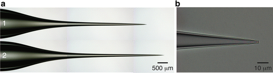
Electrode characteristics . (a) The ideal electrode has a long, tapered shank whose length is adjusted to the recording depth. Electrode 1 aims at recording from supragranular layers in rat; electrode 2 has a longer shank and allows recording from granular and infragranular layers without damaging superficial layers at point of entry. The maximal diameter of the electrode inside the brain is ~75 μm. (b) Inner diameter of electrode tip is ~1 μm, resulting in electrode resistance of 3–6 MΩ
-
Depending on the recording depth (with respect to pial surface), the taper dimensions of the recording electrode are adjusted. The taper diameter should be <75 μm at point of entry in the brain to avoid mechanical damage or stress to the recording area. For recordings in supragranular layers of rat primary somatosensory cortex , a taper of 300–500 μm with an outer diameter of maximally 75 μm suffices (Fig. 1, electrode 1) whereas recordings from granular and infragranular layers require electrodes with a taper of 600–2000 μm, again with an outer diameter that does not exceed 75 μm at point of entry (thus: at 600–2000 μm from electrode tip).
-
To target the D2 column of adolescent Wistar rat primary somatosensory cortex (P35-45), set the angle of the electrode to 34° with respect to the sagittal plane.
-
Connect the head stage to an amplifier in bridge- or current-clamp mode.
-
Position the electrode in close proximity of the craniotomy . Fill the recording chamber with 0.9 % NaCl and determine the electrode resistance by applying a square pulse of 1 nA positive current injection (200 ms on/off).
-
Apply 100–150 mbar overpressure on the recording electrode and continuously monitor the electrode resistance. Advance with 1 μm steps until the resistance increases, which reflects contact with the dura mater. At this point, set the coordinates of the micromanipulator to “zero” to allow accurate depth measurement after single-unit isolation.
-
Advance in 1 μm steps until the patch pipette penetrates the dura mater, which can be observed as a sudden drop in electrode resistance . Remove the holding pressure from the electrode.
-
Search for single units while advancing in 1 μm steps and monitor the electrode resistance continuously using square pulse current injection. Proximity and physical contact of individual neurons lead to an increase in electrode resistance. Slowly advance the electrode until positive action potential waveforms of ~2 mV are recorded.
Spiking frequencies obtained in rat somatosensory cortex across behavioral states are typically in the order of 0.1–5.0 Hz, characteristic of sparse coding [1, 40, 49, 52] although a subset of (inter)neurons have been recorded at higher spiking rates [28, 49, 53]. Regardless of spiking frequencies, the juxtasomal loose-patch recording ensures unprecedented single-unit isolation using conventional cluster cutting procedures adapted from extracellular recording methods. A signal to noise ratio of 4:1 (~2 mV spikes) allows reliable detection of spikes using MClust (David Redish, University of Minnesota, USA) based on either peak/valley or principle component analysis (PCI1 vs. PCI2). Additionally, interspike interval distributions can be plotted to confirm the presence of a refractory period of ~3 ms [54, 55], highly indicative of single-unit isolation. Single-unit isolation for electrophysiology, labeling, and reconstruction of only the recorded neuron is critical when studying the function of individual neurons in brain areas with intermingled cell types (e.g., cerebral cortex).
-
To study action potential spiking characteristics of individual units in rat primary somatosensory cortex in awake, head-restrained rats, equip the setup with high-speed videography to monitor whisker position and movement. Free whisking involves stereotypic protraction and retraction of the whiskers at 4–12 Hz [51, 56–58] which can be captured sufficiently at ~100 Hz imaging resolution . To study active object touch, a higher temporal resolution (200–500 Hz) is typically used [28, 49, 53] (Fig. 2, 200 Hz).
Fig. 2 
Juxtasomal recording of post hoc reconstructed L5B thick tufted pyramid in primary somatosensory cortex of awake, head-restrained rat. (a) Example experiment combining juxtasomal recording with high-speed videography (@ 200 Hz) to obtain single-unit spiking properties during tactile exploration. Juxtasomal recording in black, spikes indicated as individual blue bullets, whisker position is tracked off-line (in grey) and in red, windows during which whisker was in contact with object. Note that spiking frequency was increased during free whisking and active object touch. (b) Spiking profile of same neuron at increased temporal resolution before biocytin labeling . (c) Spiking profile during biocytin loading . Note the increased action potential spiking frequency during on-phase of current injections (200 ms on/off). (d) Spiking profile after biocytin loading . The recording of spontaneous activity after labeling allows recovery from high action potential frequencies associated with breaking into the neuron and excessive inflow of extracellular ions. (e) Post hoc Neurolucida reconstruction to classify recorded neuron from panels a–d (L4 barrel contour in grey). Extensive apical tuft branching is characteristic of L5B thick tufted pyramidal neuron. Thus, the procedure allows a link between physiological properties of recorded neuron during somatosensory processing to single-cell morphological identity
The combination of electrophysiology and high-speed videography captures action potential spiking synchronized to behavior. The electrophysiological data is analyzed relatively straightforward and spikes can be regarded as binary events as a first step (ignoring amplitude adaptation during bursts) . The behavioral data is much more complex and parameters on whisker use are tracked off-line [59] and can be represented as whisker position (degree), velocity (degrees/s), acceleration (degrees/s2), whisker curvature, touch times, or a multidimensional combination to correlate single-unit spiking to sensory behavior.
-
After obtaining all physiological parameters, the neuron can be biocytin labeled for post hoc identification and morphological reconstruction.
-
For juxtasomal biocytin labeling , advance the electrode until the electrode resistance is 25–35 MΩ and spikes have amplitudes of 3–8 mV to obtain optimal conditions of juxtasomal filling. Start the juxtasomal filling by applying square pulses of positive current (1 nA, 200 ms on/off). Slowly and gradually increase the current by steps of 0.1 nA while closely monitoring the action potential waveform and frequency (Fig. 2).
-
Monitor the membrane opening as a clear increase in action potential frequency during the on-phase of the block pulse (Fig. 2c). The spike waveform during filling shows an increased width and reduced after-hyperpolarization (Fig. 2c, d). Additional parameters include increased noise or a small (1–5 mV) negative DC shift [48].
-
To maintain stable biocytin infusion after opening of the membrane (reflected by robust increase in action potential frequency during on-phase of the block pulse), the amplitude of current injections can typically be reduced (1–3 nA). Stop or even further reduce the current pulses upon sudden increase of the action potential frequency (also during off-phase) to avoid toxicity by excess influx of extracellular ions.
-
Closely monitor the action potential spiking frequency after stopping the current injection. The spike waveform after a filling session is usually broadened and shows a strongly reduced after-hyperpolarization. Wait for recovery of the neuron, which is apparent when the spike waveform and action potential frequency return to its original properties (i.e., presence of normal after-hyperpolarization , Fig. 2).
-
Repeat biocytin filling sessions after complete recovery of the neuron to increase biocytin load for improved staining quality.
-
Retract the patch pipette in steps of 1 μm until the spike amplitude decreases to reduce any mechanical stress to the neuron. For cell-type identification and/or dendritic reconstructions, a typical diffusion time of 15–20 min is sufficient.
-
After biocytin labeling , take the rat out of the head-fixation apparatus and anesthetize deeply with non-gaseous anesthesia (e.g., urethane or ketamine/xylazine) for transcardial perfusion with 0.9 % NaCl and subsequent fixation with 4 % paraformaldehyde (in 0.12 M phosphate buffer).


2.4 Perfusing the Animal and Removing the Brain
-
Prepare the perfusion setup, rinse and pre-load the tubing with 0.9 % NaCl.
-
Secure the rat on a surgical tray. Ensure sufficient depth of the anesthesia; foot pinch and eyelid reflexes should be absent.
-
Make a medial to lateral incision through the abdominal wall just beneath the rib cage and proceed in posterior-anterior direction to expose the sternum. Pull the sternum in anterior direction, make a small incision in the diaphragm, cut through the lower ribs, and continue the incision along the entire length of the abdominal cavity to expose the heart.
-
Remove the pericardium.
-
Insert the needle into the left ventricle and make an incision in the right atrium. Perfuse with 0.9 % NaCl (~8 ml/min).
-
Switch the infusion to 4 % paraformaldehyde (PFA) to fix the rat until stiffness of front paw and lower jaw is apparent.
-
Decapitate the rat using a pair of scissors.
-
Trim the remaining neck muscles and expose the skull completely.
-
Position the scissors in the brain stem on the dorsal side and cut the bone carefully along the sagittal suture, maintaining the dorsal position.
-
Remove the bones from both sides of the sagittal suture to expose the brain by using a forceps. Carefully remove the dura to avoid damage.
-
Carefully insert a blunt spatula to the ventral side of the brain and remove the brain gently.
-
Post-fix the entire brain overnight in 4 % PFA at 4 °C. Switch the brain to 0.05 M phosphate buffer (PB) and store at 4 °C.
-
To slice the brain in 100 μm tangential sections, take the brain out of the 0.05 M PB and put it on a filter paper facing anterior. Use a sharp razor blade to cut off the cerebellum along the coronal plane and separate the hemispheres by cutting along the midsagittal plane.
-
Apply superglue on the mounting platform and mount the left hemisphere on its sagittal plane with anterior facing right. Secure the mounting platform at an angle of 45° on a vibratome and submerge the brain in 0.05 M PB.
-
Secure a razor blade on the vibratome and make sure that the first contact with the brain surface is in the middle of the anterior-posterior plane of the hemisphere. Cut 24 100 μm sections and collect them in a 24-well plate containing 0.05 M PB.
2.5 Histological Procedures
-
Histological protocols for the cytochrome oxidase staining and the avidin-biotin-peroxidase method are performed according to previously described methods [19, 48, 60]. Optional: visualize biocytin using fluorescent avidin/streptavidin-Alexa conjugates. This additionally allows double staining with retrograde or anterograde tracing techniques.
-
Wash sections 5 × 5 min with 0.05 M PB and prepare the 3,-3′-diaminobenzidine tetrahydrochloride (DAB)-containing solution (0.2 mg/ml CytC, 0.2 mg/ml Catalase, 0.5 mg/ml DAB in 0.05 PB) for the cytochrome oxidase staining to visualize barrels in layer 4 of primary somatosensory cortex . Incubate sections 6–12 from the pia in the preheated solution for 30–45 min at 37 °C.
-
Rinse sections with 0.05 M PB for 6 × 5 min and quench endogenous peroxidase activity by incubating all sections in 3 % H2O2 in 0.05 M PB for 20 min at room temperature (RT).
-
Rinse sections with 0.05 M PB for 5 × 10 min. Incubate sections in ABC solution overnight at 4 °C containing 0.05 M PB, 0.5 % Triton, 1 drop of components A and B/10 ml 0.05 PB (ABC Kit Vector Laboratories, Burlingame, USA).
-
Rinse sections with 0.05 M PB for 5 × 10 min and prepare the DAB solution containing 0.05 M PB, 0.5 mg/ml DAB, 0.1 % H2O2 to visualize the biocytin-filled neuron. Incubate sections in filtered solution for 45–60 min at RT.
-
Rinse sections with 0.05 M PB for 5 × 10 min Mount sections on microscope slides and cover slip with mowiol.
-
Determine labeling quality using light microscopy (Fig. 3) .
Fig. 3 
Photographs of biocytin-labeled neurons. (a1) Coronal view of a rat layer 3 pyramidal neuron with 4× objective. (a2) Same neuron as (a1) but at high magnification (100× objective). (b) Tangential view of a mouse layer 4 spiny stellate (20× objective)

3 Outlook
In conclusion, the juxtasomal recording method generates data on action potential spiking of single, identified neurons in anesthetized or awake, behaving animals. This allows careful dissection of neuronal microcircuits consisting of a wide range of cell types, for instance the cortical column, and aims to address questions on cell-type-specific function during information processing and behavioral output. At present, not only patch-clamp techniques such as juxtasomal recordings (this chapter) or the tight-seal whole-cell recording method (for instance Chaps. 1, 6 and 9 [61]) are routinely applied to study related research problems but alternative methods exist such as 2-photon imaging alone or in combination with electron microscopy reconstruction [62, 63]. In general, these methods can be highly synergistic with juxtasomal recordings since they generate information on the level of network structure and function. Briefly, whole-cell patch-clamp recordings (unlike juxtasomal recordings) are highly suitable to study spontaneous or stimulus-evoked subthreshold membrane voltage dynamics. To record these membrane potential fluctuations however, it is necessary to break into the cell and dialyze the intracellular which inherently will affect electrolyte balance and action potential generation [64]. Including biocytin in the electrode solution permits post hoc reconstruction of cellular morphology at micrometer resolution [23, 30, 65]. The 3D volume that is occupied by distally projecting axons can frequently be up to several cubic millimeters and complete reconstruction of neurons from in vivo whole-cell recordings (as well as juxtasomal recordings) thus involves relatively large volumes [66–68]. In contrast, 2P imaging and dense EM reconstruction at nanometer resolution of the imaged network exclusively involves much smaller volumes (100 s of μm3) [69]. The major advantage is obviously the possibility to study population activity and neuronal synchrony in addition to connectivity parameters at single-synapse resolution , but 2P imaging techniques are limited to optically accessible (hence superficial) brain areas and the dimensions of EM reconstructed brain tissue can never compete with reconstruction of relatively large volumes obtained with whole-cell or juxtasomal recordings. Ideally these different patch-clamp and imaging techniques are combined to reach a comprehensive understanding on the structure and function of individual neurons and/or networks. Eventually, merging data from different approaches will lead to comprehensive models on brain function and a full understanding of the cellular basis of simple behaviors [25, 43, 70–74].
References
Schubert D (2007) Observing without disturbing: how different cortical neuron classes represent tactile stimuli. J Physiol 581(Pt 1):5
Joshi S, Hawken MJ (2006) Loose-patch-juxtacellular recording in vivo – a method for functional characterization and labeling of neurons in macaque V1. J Neurosci Methods 156(1–2):37–49
Pinault D (1996) A novel single-cell staining procedure performed in vivo under electrophysiological control: morpho-functional features of juxtacellularly labeled thalamic cells and other central neurons with biocytin or neurobiotin. J Neurosci Methods 65(2):113–136
DeFelipe J (2013) Cajal and the discovery of a new artistic world: the neuronal forest. Prog Brain Res 203:201–220
Sotelo C (2011) Camillo Golgi and Santiago Ramon y Cajal: the anatomical organization of the cortex of the cerebellum. Can the neuron doctrine still support our actual knowledge on the cerebellar structural arrangement? Brain Res Rev 66(1–2):16–34
Devor A et al (2013) The challenge of connecting the dots in the B.R.A.I.N. Neuron 80(2):270–274
Markram H (2006) The blue brain project. Nat Rev Neurosci 7(2):153–160
Markram H (2012) The human brain project. Sci Am 306(6):50–55
Markram H (2013) Seven challenges for neuroscience. Funct Neurol 28(3):145–151
Armstrong-James M, Fox K, Das-Gupta A (1992) Flow of excitation within rat barrel cortex on striking a single vibrissa. J Neurophysiol 68(4):1345–1358
Mountcastle VB, Davies PW, Berman AL (1957) Response properties of neurons of cat’s somatic sensory cortex to peripheral stimuli. J Neurophysiol 20(4):374–407
Simons DJ (1978) Response properties of vibrissa units in rat SI somatosensory neocortex. J Neurophysiol 41(3):798–820
Gilbert CD, Wiesel TN (1979) Morphology and intracortical projections of functionally characterised neurones in the cat visual cortex. Nature 280(5718):120–125
Mitani A et al (1985) Morphology and laminar organization of electrophysiologically identified neurons in the primary auditory cortex in the cat. J Comp Neurol 235(4):430–447
Larkman A, Mason A (1990) Correlations between morphology and electrophysiology of pyramidal neurons in slices of rat visual cortex. I. Establishment of cell classes. J Neurosci 10(5):1407–1414
Mason A, Larkman A (1990) Correlations between morphology and electrophysiology of pyramidal neurons in slices of rat visual cortex. II. Electrophysiology. J Neurosci 10(5):1415–1428
Powell TP, Mountcastle VB (1959) Some aspects of the functional organization of the cortex of the postcentral gyrus of the monkey: a correlation of findings obtained in a single unit analysis with cytoarchitecture. Bull Johns Hopkins Hosp 105:133–162
Hamill OP et al (1981) Improved patch-clamp techniques for high-resolution current recording from cells and cell-free membrane patches. Pflugers Arch 391(2):85–100
Horikawa K, Armstrong WE (1988) A versatile means of intracellular labeling: injection of biocytin and its detection with avidin conjugates. J Neurosci Methods 25(1):1–11
Marx M et al (2012) Improved biocytin labeling and neuronal 3D reconstruction. Nat Protoc 7(2):394–407
Markram H et al (1997) Physiology and anatomy of synaptic connections between thick tufted pyramidal neurones in the developing rat neocortex. J Physiol 500(Pt 2):409–440
Feldmeyer D et al (1999) Reliable synaptic connections between pairs of excitatory layer 4 neurones within a single “barrel” of developing rat somatosensory cortex. J Physiol 521(Pt 1):169–190
Brecht M, Sakmann B (2002) Whisker maps of neuronal subclasses of the rat ventral posterior medial thalamus, identified by whole-cell voltage recording and morphological reconstruction. J Physiol 538(Pt 2):495–515
de Kock CP et al (2007) Layer and cell type specific suprathreshold stimulus representation in primary somatosensory cortex. J Physiol 581(1):139–154
Feldmeyer D et al (2012) Barrel cortex function. Prog Neurobiol 2013 Apr;103:3–27. doi: 10.1016/j.pneurobio.2012.11.002. Epub 2012 Nov 27. Review.
Mountcastle VB (1997) The columnar organization of the neocortex. Brain 120(Pt 4):701–722
Oberlaender M et al (2012) Cell type-specific three-dimensional structure of thalamocortical circuits in a column of rat vibrissal cortex. Cereb Cortex 22(10):2375–2391
Gentet LJ et al (2012) Unique functional properties of somatostatin-expressing GABAergic neurons in mouse barrel cortex. Nat Neurosci 15(4):607–612
Schubert D, Kotter R, Staiger JF (2007) Mapping functional connectivity in barrel-related columns reveals layer- and cell type-specific microcircuits. Brain Struct Funct 212(2):107–119
Brecht M, Roth A, Sakmann B (2003) Dynamic receptive fields of reconstructed pyramidal cells in layers 3 and 2 of rat somatosensory barrel cortex. J Physiol 553(Pt 1):243–265
Brecht M, Sakmann B (2002) Dynamic representation of whisker deflection by synaptic potentials in spiny stellate and pyramidal cells in the barrels and septa of layer 4 rat somatosensory cortex. J Physiol 543(Pt 1):49–70
Manns ID, Sakmann B, Brecht M (2004) Sub- and suprathreshold receptive field properties of pyramidal neurones in layers 5A and 5B of rat somatosensory barrel cortex. J Physiol 556(Pt 2):601–622
Klausberger T et al (2003) Brain-state- and cell-type-specific firing of hippocampal interneurons in vivo. Nature 421(6925):844–848
Mileykovskiy BY, Kiyashchenko LI, Siegel JM (2005) Behavioral correlates of activity in identified hypocretin/orexin neurons. Neuron 46(5):787–798
Bevan MD et al (1998) Selective innervation of neostriatal interneurons by a subclass of neuron in the globus pallidus of the rat. J Neurosci 18(22):9438–9452
Varga C, Golshani P, Soltesz I (2012) Frequency-invariant temporal ordering of interneuronal discharges during hippocampal oscillations in awake mice. Proc Natl Acad Sci U S A 109(40):E2726–E2734
Voigt BC, Brecht M, Houweling AR (2008) Behavioral detectability of single-cell stimulation in the ventral posterior medial nucleus of the thalamus. J Neurosci 28(47):12362–12367
Aksay E et al (2000) Anatomy and discharge properties of pre-motor neurons in the goldfish medulla that have eye-position signals during fixations. J Neurophysiol 84(2):1035–1049
Burgalossi A et al (2011) Microcircuits of functionally identified neurons in the rat medial entorhinal cortex. Neuron 70(4):773–786
de Kock CP, Sakmann B (2009) Spiking in primary somatosensory cortex during natural whisking in awake head-restrained rats is cell-type specific. Proc Natl Acad Sci U S A 106(38):16446–16450
Jorntell H, Ekerot CF (2006) Properties of somatosensory synaptic integration in cerebellar granule cells in vivo. J Neurosci 26(45):11786–11797
Boudewijns ZS et al (2013) Layer-specific high-frequency action potential spiking in the prefrontal cortex of awake rats. Front Cell Neurosci 7:99
Helmstaedter M et al (2007) Reconstruction of an average cortical column in silico. Brain Res Rev 55(2):193–203
Ray S et al (2014) Grid-layout and theta-modulation of layer 2 pyramidal neurons in medial entorhinal cortex. Science 343(6173):891–896
Burgalossi A, Brecht M (2014) Cellular, columnar and modular organization of spatial representations in medial entorhinal cortex. Curr Opin Neurobiol 24(1):47–54
Doron G et al (2014) Spiking irregularity and frequency modulate the behavioral report of single-neuron stimulation. Neuron 81(3):653–663
Houweling AR, Brecht M (2008) Behavioural report of single neuron stimulation in somatosensory cortex. Nature 451(7174):65–68
Narayanan RT et al (2014) Juxtasomal biocytin labeling to study the structure-function relationship of individual cortical neurons. J Vis Exp 84:e51359
O’Connor DH et al (2010) Neural activity in barrel cortex underlying vibrissa-based object localization in mice. Neuron 67(6):1048–1061
Bagdasarian K et al (2013) Pre-neuronal morphological processing of object location by individual whiskers. Nat Neurosci 16(5):622–631
Carvell GE, Simons DJ (1990) Biometric analyses of vibrissal tactile discrimination in the rat. J Neurosci 10(8):2638–2648
Barth AL, Poulet JF (2012) Experimental evidence for sparse firing in the neocortex. Trends Neurosci 35(6):345–355
Curtis JC, Kleinfeld D (2009) Phase-to-rate transformations encode touch in cortical neurons of a scanning sensorimotor system. Nat Neurosci 12(4):492–501
de Kock CP, Sakmann B (2008) High frequency action potential bursts (>or = 100 Hz) in L2/3 and L5B thick tufted neurons in anaesthetized and awake rat primary somatosensory cortex. J Physiol 586(14):3353–3364
Fee MS, Mitra PP, Kleinfeld D (1996) Variability of extracellular spike waveforms of cortical neurons. J Neurophysiol 76(6):3823–3833
Gao P, Bermejo R, Zeigler HP (2001) Whisker deafferentation and rodent whisking patterns: behavioral evidence for a central pattern generator. J Neurosci 21(14):5374–5380
Berg RW, Kleinfeld D (2003) Rhythmic whisking by rat: retraction as well as protraction of the vibrissae is under active muscular control. J Neurophysiol 89(1):104–117
Hill DN et al (2008) Biomechanics of the vibrissa motor plant in rat: rhythmic whisking consists of triphasic neuromuscular activity. J Neurosci 28(13):3438–3455
Knutsen PM, Derdikman D, Ahissar E (2005) Tracking whisker and head movements in unrestrained behaving rodents. J Neurophysiol 93(4):2294–2301
Wong-Riley M (1979) Changes in the visual system of monocularly sutured or enucleated cats demonstrable with cytochrome oxidase histochemistry. Brain Res 171(1):11–28
Sakmann B, Neher E (1995) Single-channel recording. Plenum Press, New York
Bock DD et al (2011) Network anatomy and in vivo physiology of visual cortical neurons. Nature 471(7337):177–182
Briggman KL, Helmstaedter M, Denk W (2011) Wiring specificity in the direction-selectivity circuit of the retina. Nature 471(7337):183–188
Margrie TW, Brecht M, Sakmann B (2002) In vivo, low-resistance, whole-cell recordings from neurons in the anaesthetized and awake mammalian brain. Pflugers Arch 444(4):491–498
Oberlaender M, Ramirez A, Bruno RM (2012) Sensory experience restructures thalamocortical axons during adulthood. Neuron 74(4):648–655
Bruno RM et al (2009) Sensory experience alters specific branches of individual corticocortical axons during development. J Neurosci 29(10):3172–3181
Boudewijns ZS et al (2011) Semi-automated three-dimensional reconstructions of individual neurons reveal cell type-specific circuits in cortex. Commun Integr Biol 4(4):486–488
Oberlaender M et al (2011) Three-dimensional axon morphologies of individual layer 5 neurons indicate cell type-specific intracortical pathways for whisker motion and touch. Proc Natl Acad Sci U S A 108(10):4188–4193
Helmstaedter M (2013) Cellular-resolution connectomics: challenges of dense neural circuit reconstruction. Nat Methods 10(6):501–507
Sarid L et al (2007) Modeling a layer 4-to-layer 2/3 module of a single column in rat neocortex: interweaving in vitro and in vivo experimental observations. Proc Natl Acad Sci U S A 104(41):16353–16358
Petreanu L et al (2009) The subcellular organization of neocortical excitatory connections. Nature 457(7233):1142–1145
Xu NL et al (2012) Nonlinear dendritic integration of sensory and motor input during an active sensing task. Nature 492(7428):247–251
O’Connor DH, Huber D, Svoboda K (2009) Reverse engineering the mouse brain. Nature 461(7266):923–929
Kleinfeld D, Deschenes M (2011) Neuronal basis for object location in the vibrissa scanning sensorimotor system. Neuron 72(3):455–468
Acknowledgements
I was introduced to the juxtasomal loose-patch technique by Randy Bruno (Columbia University, NY, USA) under the supervision of Prof. Dr. Bert Sakmann and thank both Randy and Prof. Sakmann for their continuous support, enthusiasm, and fruitful collaborations. Additionally, I'd like to thank Anton Pieneman for excellent technical support.
Author information
Authors and Affiliations
Editor information
Editors and Affiliations
Rights and permissions
Copyright information
© 2016 Springer Science+Business Media New York
About this protocol
Cite this protocol
de Kock, C.P.J. (2016). Juxtasomal Loose-Patch Recordings in Awake, Head-Fixed Rats to Study the Link Between Structure and Function of Individual Neurons. In: Korngreen, A. (eds) Advanced Patch-Clamp Analysis for Neuroscientists. Neuromethods, vol 113. Humana Press, New York, NY. https://doi.org/10.1007/978-1-4939-3411-9_2
Download citation
DOI: https://doi.org/10.1007/978-1-4939-3411-9_2
Published:
Publisher Name: Humana Press, New York, NY
Print ISBN: 978-1-4939-3409-6
Online ISBN: 978-1-4939-3411-9
eBook Packages: Springer Protocols