Secondary Metabolic Pathway-Targeted Metabolomics

Abstract

This chapter provides step-by-step methods for building secondary metabolic pathway-targeted molecular networks to assess microbial natural product biosynthesis at a systems level and to aid in downstream natural product discovery efforts. Methods described include high-resolution mass spectrometry (HRMS)-based comparative metabolomics, pathway-targeted tandem MS (MS/MS) molecular networking, and isotopic labeling for the elucidation of natural products encoded by orphan biosynthetic pathways. The metabolomics network workflow covers the following six points: (1) method development, (2) bacterial culture growth and organic extraction, (3) HRMS data acquisition and analysis, (4) pathway-targeted MS/MS data acquisition, (5) mass spectral network building, and (6) network enhancement. This chapter opens with a discussion on the practical considerations of natural product extraction, chromatographic processing, and enhanced detection of the analytes of interest within complex organic mixtures using liquid chromatography (LC)-HRMS. Next, we discuss the utilization of a chemometric platform, focusing on Agilent Mass Profiler Professional software, to run MS-based differential analysis between sample groups and controls to acquire a unique set of molecular features that are dependent on the presence of a secondary metabolic pathway. Using this unique list of molecular features, the chapter then details targeted MS/MS acquisition for subsequent pathway-dependent network clustering through the online Global Natural Products Social Molecular Networking (GnPS) platform. Genetic information, ionization intensities, isotopic labeling, and additional experimental data can be mapped onto the pathway-dependent network, facilitating systems biosynthesis analyses. The finished product will provide a working molecular network to assess experimental perturbations and guide novel natural product discoveries.

1 Introduction

Microbial genome sequencing efforts are illuminating a growing number of “orphan” biosynthetic gene clusters suspected of biosynthesizing novel natural products with pharmacological, agricultural, and biotechnological values [1]. These unknown small molecules possess the potential to serve as new molecular probes, dietary supplements, flavors, fragrances, signaling agents, commercial products, drugs, and drug leads [2]. Unfortunately, the valuable products of most orphan pathways remain “cryptic,” “silent,” or simply undetectable in the laboratory environment, undercutting discovery efforts. This chapter describes a “pathway-targeted” structural networking approach, which can be used to aid in the detection and elucidation of these important small molecules known as secondary metabolites (Fig. 1).

Fig. 1

Untargeted versus pathway-targeted mass spectral data collection. Under untargeted MS /MS fragmentation modes, abundant ions are preferentially selected for fragmentation (highlighted with stars), and depending on inclusion and exclusion parameters, many of the less abundant ions go undetected in MS/MS data. Under pathway-targeted fragmentation modes, only pathway-dependent masses are selected (highlighted in red and by stars), providing higher fragmentation coverage of the secondary metabolic pathway ions of interest for subsequent molecular networking

Secondary metabolites from microorganisms are most often encoded by biosynthetic gene clusters, including nonribosomal peptide synthetase (NRPS ) and polyketide synthase (PKS ) systems, among others. Mass spectrometry (MS ) and tandem MS (MS/MS) techniques are important tools in secondary metabolite detection, discovery, and characterization. Secondary metabolic pathways often produce a series of structurally related intermediates and products, and consequently, the MS/MS fragmentation data can be used to organize and delineate related molecules into network clusters or “molecular families” [3, 4]. Employing these foundational molecular networking tools developed by Dorrestein and coworkers [3, 4], we recently developed a “pathway-targeted” structural networking approach (Fig. 2) to finely map a bacterial secondary metabolic pathway found in the human gut and linked to colorectal cancer initiation [5, 6]. A defining feature separating microbial secondary metabolism, which is typically involved in host virulence, pathogenicity, mutualism, antibiotic production, and diverse chemical signaling events, from primary metabolism is the general ability to cleanly delete a metabolic pathway from a cell while retaining cell growth and avoiding many of the complications due to primary metabolic rerouting. Consequently, comparative metabolomics analysis among controls, wild-type organisms, and pathway mutant organisms (or heterologous expression systems) can be used to map molecular features dependent on functional pathways (Fig. 3). Here, we use the raw data from our recent studies on the bacterial colibactin pathway to illustrate pathway-targeted structural networking (Methodology Overview, Fig. 2) [5, 6], which can be applied to the majority of secondary metabolic pathways of interest in genetically tractable production hosts.

Fig. 2

Workflow overview for pathway-targeted molecular networking

Fig. 3

Pathway-targeted mass spectral networking. (a) An untargeted auto MS /MS approach leads to a network with a much larger number of total ion masses (nodes) with often more limited coverage of less abundant pathway-dependent ions. As highlighted in the Venn Diagram, there are a large number of entities associated with controls (media components, primary metabolites, and contaminants). (b) By removing all entities detected in any control sample, targeted MS/MS can be performed to access higher MS/MS fragmentation coverage for “pathway-dependent” molecular features (MOFs) associated with the presence of the gene cluster of interest (highlighted in Venn Diagram)

2 Materials

Prepare all culture media and solutions using Milli-Q ultrapure water. High-performance liquid chromatography (HPLC) grade solvents should be used for organic extractions, and LC-MS grade water and solvents should be used for all Q-TOF MS analyses.

2.1 Culture Growth and Extraction

• 1. General lysogeny broth (LB) or LB agar, Miller (see Note 1 ).

• 2. Difco M9 minimal medium supplemented with casamino acids (5 g/L), 0.4 % (w/v) glucose (filter-sterilized, store at 4 °C until use), 2.0 mM magnesium sulfate (MgSO₄, sterile), and 0.1 mM calcium chloride (CaCl₂, sterile) (see Note 2 ). Add antibiotic(s) to sterile medium if needed.

• 3. Isopropyl β-d-1-thiogalactopyranoside (IPTG), aqueous stock solution: 1.0 M filter-sterilized and stored in aliquots at −20 °C.

• 4. Petri dish (100 × 15 mm).

• 5. Polypropylene culture tubes (14 mL) (see Note 3 ).

• 6. Glass serological pipettes.

• 7. 16 × 100 mm disposable test tubes, borosilicate glass.

• 8. Ethyl acetate, HPLC grade (see Note 4 ).

2.2 Amino Acid Isotope-Labeled Culture Growths

• 1. Isotopically labeled l-amino acids (e.g., [U-¹³C₃]-l-Cys) (see Note 5 ).

2.3 LC-MS Analysis

• 1. Polypropylene LC-MS vials, 250 μL (see Note 6 ).

• 2. Methanol, LC-MS grade.

• 3. Mobile phase A: LC-MS grade water with 0.1 % formic acid.

• 4. Mobile phase B: LC-MS grade acetonitrile with 0.1 % formic acid.

• 5. Phenomenex Kinetex™ 1.7 μm C18 100 Å LC column (100 × 2.10 mm) or comparable analytical ultrahigh-performance LC column (see Note 7 ).

• 6. HPLC system: Agilent 1290 Infinity Binary HPLC system equipped with Diode Array Detector, autosampler, or comparable system.

• 7. Mass spectrometer: Agilent 6550 iFunnel quadrupole time-of-flight (Q-TOF) MS instrument equipped with a Dual Agilent Jet Stream (AJS) electrospray ionization (ESI ) source, running in positive mode (or negative mode) scanning from 25 to 1700 m/z mass range at 1.00 spectra/s or comparable instrument and conditions.

• 8. Agilent MS standard reference mass solution: m/z 121.05087300 (purine) and m/z 922.00979800 (hexakis (1H, 1H, 3H-tetrafluoropropoxy)phosphazene).

• 9. Software: MassHunter Workstation Data Acquisition (Agilent Technologies), MassHunter Qualitative Analysis (Agilent Technologies), and Mass Profiler Professional (Agilent Technologies).

3 Methods

Comparative metabolomics analysis should be conducted at least between a biological control group (described below) and a wild-type sample group expressing the secondary metabolite pathway of interest; mutated derivatives of the pathway can be included. The conditions described below are for Escherichia coli strains heterologously expressing a representative hybrid NRPS -PKS biosynthetic gene cluster under an IPTG-inducible system. Correspondingly, the protocols can be modified if the gene cluster is expressed natively or under other inducible systems and should transfer well to other genetically tractable production hosts. Methods can be modified based on growth requirements for different bacterial systems. Once the conditions have been selected for a given pathway, use the same methods when performing growths and organic extractions within a metabolomics experiment to minimize variables and disparities that can influence data analysis. Selection of biological controls is important when designing your experiment. As a biological control, we recommend using the bacterial strain with the full gene cluster deleted to maximize characterization of pathway-dependent metabolites during analysis. Alternatively, deletion of a selected core biosynthetic gene would suffice. Following a systematic approach, method development should involve three main aspects: (1) extraction method, (2) LC method, and (3) MS detection method. As an example, extraction of whole culture metabolomes (cells plus supernatant) by ethyl acetate is described below (see Note 8 ).

3.1 Bacterial Growth and Organic Extraction

• 1. Streak bacteria from frozen stock (stored at −80 °C) onto LB agar plate (with necessary antibiotic(s)). Incubate overnight at 37 °C or until single colonies are formed (see Note 9 ).

• 2. Inoculate 5 mL LB (with appropriate antibiotic(s)) in a polypropylene culture tube with one single colony as a seed culture. We recommend a total of five biological replicates. Incubate while shaking (250 rpm) at 37 °C for 12–14 h (see Note 10 ).

• 3. Next day, inoculate 5 mL M9 minimal broth (with appropriate antibiotic(s)) in a polypropylene culture tube with overnight seed culture (1:100). Grow at 37 °C (250 rpm) until optical density (OD₆₀₀) is 0.5 for inducible systems (see Note 11 ). Place culture at 4 °C for 10 min before induction (if necessary). Then add IPTG to the desired concentration and allow cultures to grow for 48 h at 25 °C, 250 rpm (see Note 12 ).

• 4. After 48 h (or designated time point), remove cultures from shaker. Add 6 mL of ethyl acetate directly onto the culture in the polypropylene tube. Cap tube tightly and vigorously shake for 30 s. Centrifuge cultures at 4 °C for at least 15 min (2800 × g). Carefully remove tubes, and transfer 4 mL of the organic layer into glass vials. Evaporate to dryness under reduced pressure. Once dried, store extracts at −20 °C until use.

3.2 LC-MS Analysis

• 1. Prepare samples for LC-MS analysis based on recommended concentration for instrument sensitivity. For the Q-TOF MS system described (Materials Section), dissolve extracted samples in 2.5 mL methanol as a starting point (see Note 13 ). Filter samples (see Note 14 ). Place 50 μL of sample in HPLC vials for analysis, dry the remaining sample volume, and store at −20 °C for future use.

• 2. Create an LC and MS method for LC-MS analysis.

  • (a) General LC method. Using mobile phase A and B, set up method as follows: 95 %/5 % A/B, 2 min; run gradient from 95 % A to 98 % B until 26 min (see Note 15 ). Hold for 5 min at 98 % B and then bring back to starting conditions. Recommended flow rate for UHPLC column described in Materials is 0.3 mL/min. Equilibrate column for recommended time (see Note 16 ).

  • (b) General MS method. Set source parameters as follows: gas temperature at 225 °C and flow at 12 mL/min, nebulizer at 50 psig, sheath gas temperature at 275 °C, and flow at 12 L/min. Set scan source parameters as follows: capillary 3500 V, fragmentor 125 V, skimmer 65 V, and OCT RF Peak 750 V.

• 3. Calibrate and tune your high-resolution mass spectrometer according to the specific settings for metabolomics analysis (see Note 17 ).

• 4. Prepare LC column by performing multiple column washes, and run LC method without an injection. Then set up workflow as follows: blank control (using same solvent used to dissolve samples), control extracts, and sample extracts. Run a blank wash between each sample set.

• 5. Place samples in autosampler, kept at 4 °C. Inject 3–5 μL based on sample concentration. Create a worklist and run samples (see Note 18 ).

3.3 Acquiring Molecular Features

• 1. First, determine quality of data using the MassHunter Qualitative Analysis program. Overlay chromatograms for each sample set to confirm system repeatability (see Note 19 ).

• 2. Then, process centroid MS data in MassHunter Qualitative Analysis. To do this, go to “Method” and create a method using the Extract Molecular Features protocol (Fig. 4). Recommended settings are outlined in Table 1 (see Note 20 ).

  Fig. 4

  

  Find compounds by molecular feature. As described in Table 1 and detailed in the chapter, the different settings (tabs) can be modified to optimize for the in silico extraction of compounds of interests

  Table 1 Recommended settings for Extract Molecular Features protocol

• 3. Open DA Reprocessor (offline program), and set up a sample worklist by clicking “Insert multiple samples.” Select samples to be analyzed, and load. Select “Method” created in step 2. Click the “Start” icon to process data. This feature will generate compound exchange format (CEF) files for all samples, which are used for differential and statistical analysis (see Note 21 ).

3.4 Statistical Analysis Using Mass Profiler Professional (MPP) (See Note 22 )

• 1. Open MPP and create a new Project.

• 2. Create new experiment (you can have multiple experiments per Project), select “combined (identified + unidentified)” experiment type, and “Data Import Wizard” as the workflow type. This is a good starting point for differential analysis by providing full guidance.

• 3. Select program used to acquire data (e.g., MassHunter Qual). Choose organism if applicable.

• 4. Upload CEF files by selecting “Select Data Files” tab. Then, create grouping for each sample set (i.e., control, wild type, and mutants) by selecting the “Add Parameter” tab.

• 5. Adjust filters as deemed necessary. Recommended initial parameter for small molecule metabolomics are “Minimum Absolute abundance” set at 5000 counts and “Minimum number of ions” set at two; Select “Multiple charge states forbidden.” At this point, it is recommended that you use all available data.

• 6. Next, set any alignment parameters necessary to align compounds in different samples if their accurate mass and retention times (RTs) fall within the specified tolerance window. Unless you are using an internal standard, recommended parameters are RT window = 0.1 % + 0.15 min and Mass window = 5.0 ppm + 2.0 mDa.

• 7. The next window shows a summary of data and provides the number of aligned compounds. Continue through the windows until analysis is finished. Once data is uploaded, perform grouping and analysis of data using the Workflow panel (right side of screen). Familiarize yourself with the different tabs within this panel.

• 8. To group samples.

  • (a) First, create a “Control” (absent/nonfunctional gene cluster) interpretation. Under “Experiment Setup,” select “Create Interpretation.” Deselect any conditions that are not a control; select “Non-Averaged,” and deselect “Absent.” Name your new parameter (e.g., Control) and click “Finish.”

  • (b) Next, create a “Sample” (with gene cluster) interpretation for wild type and mutant(s), individually, as specified in step 8a. Once you are done, the newly created interpretations can be seen on the left panel under your experiment. At this point, there should be one interpretation from each sample set (i.e., control, wild type, mutant, etc.).

• 9. To perform analysis.

  • (a) First, do analysis on control samples. Go to the “Quality Control” tab in the Worklist Panel, and select “Filter by Abundance.” In the “Entity List” tab, select “All Entities.” Under the “Interpretation” tab, select the control interpretation. Under “Retain entities in which” section, select at least “1” out of the 5 samples that have values within range (see Note 23 ). Name your analysis and click “Finish.”

  • (b) Perform a stricter analysis on samples that contain the pathways. Do the same as was done for the control using the “Filter by Abundance” analysis. But, under “Retain entities in which” section, select at least “5” out of the 5 samples that have values within range (see Note 24 ).

• 10. Next, create a Venn Diagram of samples to be compared. Go to “Tools,” and under “Venn Diagram,” select “Entity List.” Conversely, click on the “Venn Diagram” icon. Select control, wild type, and mutant samples and click “OK” (Fig. 3a, Venn Diagram).

• 11. Create a new entity list of molecular features only found in samples with pathway by highlighting the respective section of the Venn Diagram (e.g., the section that corresponds only to wild type). Select the “Create Entity List” icon (icon of Page with pencil). Confirm that entities found only in desired sample are selected, then save new entity list.

• 12. Repeat step 11 as many times as necessary (for each desired sample group, e.g., wild type, mutant 1, mutant 2, etc.) to acquire a conservative unique entity list consisting of pathway-dependent molecular features. Molecular features found in all sample strains (with pathway) can be compared (Fig. 3b, Venn Diagram).

• 13. Examine each unique list, and confirm that ions are not found in control samples (do this in MassHunter Qualitative Analysis software) (see Note 25 ). To export molecular feature list into Excel files do as follows:

  • (a) Export inclusion list using the tab under “Workflow/Results Interpretation” panel. Save the output file and select “next.” On the subsequent page, select the following parameters: (1) limit number of precursor per compound to 1 ion(s); (2) export highest abundance m/z, (3) positive ions [H] and [Na]. The resulting list contains the ion masses to be fragmented and will be used as the precursor list for MS /MS fragmentation.

  • (b) To download the HRMS, retention time, and abundance (raw and normalized) information, right-click the data file of interest. Select “Export list” option, select the information you want to download (e.g., raw abundance, normalized abundance, mass, retention time), and create file.

3.5 MS /MS Fragmentation

• 1. Prepare samples for LC-MS /MS analysis as was done in Subheading 3.2, and prepare system using same calibration MS conditions and LC method.

• 2. Create a MS /MS method by selecting the “Auto MS/MS” setting. At this point, an untargeted metabolomics data set can be collected by performing an “Auto MS/MS” run (see Note 26 ).

• 3. To run a pathway-targeted metabolomics experiment, specifically target masses from the unique ion list. In the Agilent system, in the “Auto MS /MS” setting under the “Preferred/Exclude” tab of the Q-TOF Acquisition section, the preferred ion list can be inserted. Right-click anywhere on the table and upload the exclusion list acquired in MPP. Change the “Delta m/z (ppm)” tab to 0.5 (depending on accuracy of system). Check the “Use Preferred ion list” box.

• 4. Create different MS /MS methods to enhance overall MS/MS data collection (see Note 27 ). Use different isotope models (under “Spectral Parameters” tab) and analyze different collision energies (e.g., 10, 20, 40) (see Note 28 ).

• 5. Prepare LC column by performing multiple washes. Then set up workflow for sample extracts to be analyzed. Place samples in autosampler, kept at 4 °C. Inject 3–5 μL based on sample concentration. Run samples.

3.6 Pathway-Targeted Mass Spectral Molecular Networking (See Note 29 )

• 1. Download the following programs: MSConvert (ProteoWizard tool) (see Note 30 ), Insilicos (see Note 31 ), and the open-source platform Cytoscape (see Note 32 ).

• 2. Convert raw MS /MS data in MSConvert to mzXML files. Use same settings as shown in Fig. 5. Open converted files and confirm correct conversion in the Insilicos program.

  Fig. 5

  

  MS convert settings. MS convert program is used to convert mass spectral data files to CEF files for analyses in Mass Profiler Professional. Selection settings are highlighted (red ovals). Once the filter is selected, click “Add,” then select “Start”

• 3. Go to GnPS (Global Natural Products Social Molecular Networking) (www.gnps.ucsd.edu), create a free account, and click on “Data Analysis” (see Note 29 ).

• 4. In the “Workflow Selection,” create a descriptive title, and upload files via a FTP connection (see Note 33 ). The host name is ccms-ftp01.ucsd.edu, and the username and password are the same as your created account.

• 5. Select spectrum file(s) to be analyzed and upload. Set parameters for the network including parent mass tolerance (0.1–2.0 Da) and min pairs cos (0.1–1.0) (see Note 34 ). For “Minimum Cluster Size,” type “1.” Perform different networks and analyze how each setting affects the clusters.

• 6. Once the analyses are finished, click “View All Clusters with IDs” and download the files.

• 7. In Cytoscape, import the “networkedges” file. Select “Column 1” under “Select Source Node Column” and “Column 2” under “Select Target Node Column.” Click “Column 3” and “Column 5” to activate (turns blue). Rename columns 3 and 5 as “deltaMZ” and “cosine,” respectively. Click OK to load the network. Select “Apply Preferred Layout” to view your initial network template (see Note 35 ).

• 8. Next, load the information parameters by importing table file “clusterinfosummarygroup_attributes_withIDs.” Deselect any columns not needed and click “OK.”

• 9. Under the Control Panel, select the “Style” tab. Here you can set different parameters to enhance the appropriate data features for the “node” or “edge” properties.

  • (a) To highlight the connectivity strength between ion masses and load cosine settings. To do this, select the “Edge” tab. For the “width” setting, select cosine for the “Column” and Continuous Mapping for the “Mapping Type.” Double-click the box, and set the min. and max. values to assess the display. The bolder (thicker) edges display stronger connectivity between ion masses.

  • (b) Load the respective masses onto each node (Fig. 3b). In the “Node” tab, under the “Label” setting, select parentmass for the “Column” and Passthrough Mapping for the “Mapping Type.”

  • (c) To distinguish between genetic variants, “node” properties can be modified. Set a distinct node shape (under “Shape”) for a specific strain source (e.g., wild type, mutant(s), all) as shown in Fig. 3b.

  • (d) To highlight differences in parent ion ionization intensities, display each strain metabolite abundances based on a heat-map coloration (Fig. 6a). To accomplish this, first go to the “Table Panel,” and manually type in the average raw abundance of each parent ions obtained for each specific strain from the MPP program (see Subheading 3.4, step 13b). For example, for the wild-type metabolite intensities, manually type in under the “sum (precursor intensity)” column the raw abundance for each unique molecular features. If a feature was not detected in the wild type, type “0.” Then select “Fill Color,” and perform a “Discrete Mapping” coloration based on the “sum (precursor intensity)” column. Save the network under a different name. Then repeat for each mutant strain, each time saving as a distinct network (Fig. 6a).

    Fig. 6

    

    Molecular network feature enhancement. (a) Features, such as average ionization intensities and other experimental data, can be used to enhance the network in Cytoscape to help guide pathway and secondary metabolite characterization. These graphical illustrations allow for the quick identification of metabolic “bottlenecks” in secondary metabolism, such as for a pathway mutant. (b) Ion masses (or molecular features, nodes) incorporating labeled amino acid (e.g., methionine (Met) or cysteine (Cys)), as determined by HRMS, are color coded on the network map. Figure was adapted from Vizcaino and Crawford [6]

3.7 Structural Characterization Support by Isotope-Labeled Feeding Experiments

• 1. Growth of cultures, organic extraction, and HRMS analysis should be performed as per previous sections (Subheadings 3.1 and 3.2) with few modifications.

• 2. First, make M9 minimal medium to account for labeled compound, which in the example given, are amino acids. In place of casamino acids, individually add the l-amino acid composition at 5 g/L total concentration as follows: 3.6 % Arg, 21.1 % Glu, 2.7 % His, 5.6 % Ile, 8.4 % Leu, 7.5 % Lys, 4.6 % Phe, 9.9 % Pro, 4.2 % Thr, 1.1 % Trp, 6.1 % Tyr, 5 % Val, 4 % Asn, 4 % Ala, 4 % Met, 4 % Gly, 4 % Cys, and 4 % Ser. Use this media for control cultures.

• 3. To incorporate isotopically labeled (¹³C/¹⁵N/²H) amino acids into products from NRPS -PKS pathways, modify above media by adding the isotope-labeled amino acid at a specific ratio for a given strain.

  • (a) For E. coli heterologous expression, auxotrophic strain variants can be used by transforming the expression plasmid or bacterial artificial chromosome containing the gene cluster of interest into the appropriate mutant strain (see Note 36 ). Growth media should then be supplemented with a 1:1 (¹²C:¹³C) ratio of nonlabeled/labeled amino acid. For example, add 2 % Cys and 2 % l-[U-¹³C]-Cys.

  • (b) If an auxotrophic variant is not available, supplement growth media with a 100 % labeled amino acid (e.g., 4 % l-[U-¹³C]-Cys).

• 4. Grow three 5 mL biological replicates per strain using the same growth conditions defined in Subheading 3.1.

• 5. After 48 h (or designated time point), remove cultures and extract with ethyl acetate. Dry organic layer as described above, then resuspend in 2.5 mL methanol (see Note 37 ), and analyze 3–5 μL by LC-Q-TOF-HRMS (as detailed in Subheading 3.2) scanning from m/z 25 to 1700.

• 6. Determine incorporation of labeled amino acid (or other compound) by examining the unique molecular features acquired from MPP.

• 7. Repeat-labeled feeding experiment in triplicate with only the labeled amino acid (e.g., 4 % l-[U-¹³C]-Cys) to confirm dose-dependent incorporation.

• 8. Label mass spectral molecular network to represent incorporation of labeled compound (e.g., l-[U-¹³C]-Cys incorporation) (Fig. 6b).

4 Notes

• 1. Miller LB broth and LB agar can be purchased as a premade mix and prepared as per the manufacturer’s instructions. We recommend that once the media source is selected, the same brands should be maintained throughout experiment sets.

• 2. These are typical components for growth of heterotrophic bacteria. Sometimes it is necessary to add other components, such as metals (e.g., Fe²⁺, Cu²⁺) or vitamins, depending on requirements for production of secondary metabolites. It is recommended that you test various cultivation conditions to optimize production of relevant metabolites (e.g., see ref. [7]).

• 3. Polypropylene culture tubes are fairly resistant to various extraction solvents including ethyl acetate, butanol, and methanol. Do not use polystyrene culture tubes.

• 4. For our representative NRPS -PKS pathway, ethyl acetate is routinely used for the enrichment of its relatively nonpolar metabolites. More polar solvents such as butanol or methanol can be used instead to enrich for more polar compounds (see Note 8 ).

• 5. For our representative NRPS -PKS pathway, amino acid incorporation provided additional structural support for all detectable pathway-dependent small molecules. It might be necessary to utilize other labeled substrates, such as uncommon amino acids. Modify experiment as appropriate in a case-by-case basis.

• 6. Based on your instrument system, make sure to get the correct vials that fit the autosampler. For the Agilent system, we use Agilent vials and caps. Always tightly cap your vials to minimize solvent evaporation during data acquisition.

• 7. The selection of stationary phase for HPLC analysis will vary depending on the type of molecules being analyzed. As a starting point, reverse-phase C18 columns work well for a median combination of polar and nonpolar compounds. For less polar compounds, a reverse-phase C8 column might be useful. For more polar compounds, Hypercarb porous graphitic carbon (PGC) columns retain polar compounds well.

• 8. Enrichment of desired secondary metabolites can be optimized through the organic extraction of different culture components (i.e., supernatant, cell, or whole culture) and/or through the use of different extraction solvents (Fig. 7). Most secondary metabolites are produced inside the cells and can be subsequently secreted into the supernatant. If the desired metabolites are found at higher concentrations in the supernatant or cell fraction, it is best to extract the desired culture component as an initial enrichment step. In that case, whole culture should be centrifuged for 15 min at 2800 × g. Filter the supernatant into a new polypropylene culture tube and perform extraction. Conversely, if cells are the desired starting material, carefully remove any leftover supernatant from the culture tube containing the cells, and then perform an organic extraction on the cell pellet. Dichloromethane or ethyl acetate solvents are routinely used in natural product isolation for the enrichment of nonpolar compounds and can be used in a solvent-solvent extraction with supernatant/whole culture. Similarly, butanol will enrich for medium polarity compounds through a solvent-solvent extraction of the whole culture or supernatant. Be aware that butanol is slightly miscible with water, so there will be a volume reduction in the top organic layer. Some small molecules are very polar and not extractable with ethyl acetate or butanol. At this point, a methanol extraction might be needed. Since water and methanol are miscible, the whole culture (or supernatant) should be lyophilized before methanol extraction. Once completely dry, add 1 mL methanol and sonicate for 5 min. Centrifuge extract for at least 15 min at 4 °C (2800 × g). Very carefully, remove culture tubes from centrifuge, take a fixed volume aliquot of the methanol extract, making sure not to disturb the pellet, and filter. Dry the filtered extract and store at −80 °C until analysis. Conversely, bacterial cells can be extracted with methanol following same procedure.

  Fig. 7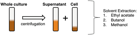

  

  Schematic for bacterial culture extraction

• 9. Select single colonies as biological replicates for analyses. Adjust cultivation time for selected organism as needed.

• 10. Secondary metabolites are often, but not always, upregulated as the cells transition to stationary phase.

• 11. OD₆₀₀ range can be between 0.45 and 0.55. We sometimes observe discrepancies between control and sample growth rates, which require cultivation time correction.

• 12. The method describes the use of an IPTG-inducible system, where IPTG serves to activate transcription of the pathway of interest. If your system is natively expressed, or under the control of another inducible system, this step is not necessary. IPTG induction and growth conditions can be optimized to increase production of small molecules of interest. We have observed that depending on gene cluster, IPTG concentrations can profoundly affect small molecule production. As a good starting range, test 0.05, 0.1, 0.25, 0.5, and 1.0 mM final concentrations to determine optimal metabolite production conditions. Other growth conditions that can be optimized include oxygenation (e.g., shaker revolutions per minute), temperature (typical range from 16 to 30 °C), or growth time, among others.

• 13. Samples prepared for HRMS instruments, such as the Agilent 6550 Q-TOF HRMS , can detect concentrations in the pg/mL range. Start at lower concentrations initially, and determine what concentrations work best for your extracts. High concentrations of a complex sample can saturate the mass detector and result in lower sensitivity or ion suppression [8, 9]. Low injection volumes of polar solvents will not greatly affect the chromatography, but high injection volumes can affect compound elution times.

• 14. To filter small quantities of sample (50 μL), pass sample through 10 μL filter tips, and collect the flow through.

• 15. To shorten run, reduce gradient time of LC method. Some ethyl acetate extracts contain nonpolar compounds; therefore, we frequently use a longer 98 % B wash.

• 16. LC column equilibration times are dependent on the column dimensions. Generally, a column should be flushed with 20 column volumes to ensure equilibration. Table 2 provides column volumes for common analytical column dimensions assuming average pore volume of 0.70. This information can be found online if dimensions are different from the ones described (e.g., see http://www.chiralizer.com/colvol.htm).

  Table 2 Some typical column dimensions and column volumes

• 17. Calibration should always be performed when changing the instrument state, and we recommend doing it before any metabolomics experiment. General calibration/tuning for the 6500 Series Q-TOF (Agilent) are as follows: (a) Set instrument to 2 GHz, EDR, low mass range for metabolomics (25–1700 m/z). (b) Calibrate in Hi Res mode, in positive or negative mode. Residual error should be less than 1 ppm. Save calibration. Reference ions spectrum should have intensity around two to three million counts. (c) Perform a standard tune (Hi Res mode), and save tune file. (d) Next, recalibrate in positive and negative mode for low masses. Re-save file as a newtunefile.tun.

• 18. Always make sure that the LC column is intact (no leaking), and check quality of data to confirm that the correct settings are being used.

• 19. Make sure that TIC chromatography is reproducible among biological replicates. If gross differences can be detected in TIC traces, start over and make sure that column equilibration times are sufficient.

• 20. The molecular feature extraction algorithm automatically retrieves all spectral information for each component, including but not limited to mass, retention time, abundance, and composite spectrum, in a sample mixture, including those in overlapping and co-eluting peaks.

• 21. We recommend using the offline DA Reprocessor program, as the Qualitative method in MassHunter Qualitative Analysis will take longer time and will require higher computing power.

• 22. MPP is a chemometric platform that can extract information from chemical systems and use the high-content mass spectral data in differential analysis to determine relationships among sample groups. MPP allows for the analysis of spectral features by importing and organizing data, identifying unique molecular features in all samples, and removing any found in sample controls and from samples lacking the gene cluster of interest.

• 23. This step compiles all molecular features detected in any control sample. The total number of control samples will vary depending on sample set, but it should include at least the five biological control replicates (without a functional gene cluster) and the solvent control runs. Any feature found in a control sample will be removed from samples (with gene cluster) in future analysis.

• 24. This selection helps to maintain a conservative analysis by only retaining the entities found in a biological sample set. This number could vary depending on the number of biological replicates. A conservative unique list for each pathway-containing sample will be built by removing any MOF found in at least one of the control replicates (no gene cluster) and keeping those that are present in all biological replicates. The strictness of the analysis can be softened by selecting for entities that are found in <“5” of the biological samples. This will tend to increase your “unique feature list” but can be used as a tool to find minor metabolites that might be under the detection limit of the sampling methodology.

• 25. We also recommend confirming mass-to-charge of each ion in the final network. We occasionally observe a very small percentage of false positives, minor abundance ions that are also found in controls, and these are removed in this final confirmation.

• 26. “Auto MS /MS” data can be used to create an untargeted mass spectral network (Fig. 3a). Method development and network construction can be performed in the same manner as is described for the data set collected for the pathway-targeted mass spectral network.

• 27. Depending on small molecules of interest and their molecular weights, different collision energies and isotope models might work best, as settings can affect selection of ions to fragment by the software. Be aware that low-abundance ions might not fragment regardless of method conditions resulting in less than 100 % coverage. Also, some secondary metabolites are unstable and may degrade before MS /MS analysis. If this is the case, re-extract fresh cultures and immediately perform MS/MS analysis.

• 28. Stronger collision energies are generally needed to effectively fragment higher molecular weight metabolites.

• 29. General Mass Spectral Molecular Networking is described in great detail in GnPS (Global Natural Products Social Molecular Networking) platform (gnps.ucsd.edu). We strongly recommend searching through their online “GnPS documentation page” for detailed information. Familiarize yourself with the different hyperlinks.

• 30. MSConvert converts original data files into mzXML files that can be uploaded for networking analysis. To acquire MSConvert, install ProteoWizard “Windows (includes vendor reader support)”; http://proteowizard.sourceforge.net/downloads.shtml.

• 31. Insilicos is a life science software that allows you to view the mzXML files and confirm that they were converted correctly. Download program from www.insilicos.com.

• 32. Cytoscape is used to view the networks created on GnPS. Download program from www.cytoscape.org.

• 33. There are various free FTP programs available online as further described in the GnPS website.

• 34. Given settings are imputed when you start the analysis, but can be modified, Parent mass tolerance setting should be set depending on your instruments’ high-resolution data. We routinely see <5 ppm error among our parent masses, and therefore, we set a lower Da error than the given setting (2.0 Da). Cosine setting dictates the connectivity strength between ion masses (similarity of fragment ions). For example, a cosine of 0.0 indicates that the ion masses are not related, while a cosine of 1.0 indicates that the ion masses are identical. In this workflow, we often build clusters based on the less conservative cosine cutoff of 0.5 (Fig. 3).

• 35. Further detailed information and properties of the Cytoscape software can be found on the GnPS documentation site.

• 36. For isotopic labeling experiments, E. coli auxotrophic variant strains from the Keio collection can be acquired from the Coli Genetic Stock Center (CGSC, Yale University, New Haven, CT, USA; http://cgsc.biology.yale.edu/) or other collections. Use of auxotrophic strain backgrounds is very helpful in data analyses, as the relative label:nonlabel substrate ratio is conserved in the parent ions of, for example, an amino acid-labeled nonribosomal peptide.

• 37. Performing a 1:1 incorporation of nonlabeled/labeled substrate will decrease overall abundance of ions of interest. Modify concentrations as deemed necessary for HRMS analysis.

References

Cimermancic P, Medema MH et al (2014) Insights into secondary metabolism from a global analysis of prokaryotic biosynthetic gene clusters. Cell 158:412–421
Newman DJ, Cragg GM (2012) Natural products as sources of new drugs over the 30 years from 1981 to 2010. J Nat Prod 75:311–335
Watrous J, Roach P, Alexandrov T et al (2012) Mass spectral molecular networking of living microbial colonies. Proc Natl Acad Sci U S A 109:E1743–E1752
Nguyen DD, Wu CH, Moree WJ et al (2013) MS/MS networking guided analysis of molecule and gene cluster families. Proc Natl Acad Sci U S A 110:E2611–E2620
Vizcaino MI, Engel P, Trautman E et al (2014) Comparative metabolomics and structural characterizations illuminate colibactin pathway-dependent small molecules. JACS 136:9244–9247
Vizcaino MI, Crawford JM (2015) The colibactin warhead crosslinks DNA. Nat Chem 7:411–417
Bode HB, Bethe B, Hofs R et al (2002) Big effects from small changes: possible ways to explore nature’s chemical diversity. Chembiochem 3:619–627
Choi BK, Hercules DM, Gusev AI et al (2001) LC-MS/MS signal suppression effects in the analysis of pesticides in complex environmental matrices. Fresenius J Anal Chem 369:370–377
Furey A, Moriarty M, Bane V et al (2013) Ion suppression; a critical review on causes, evaluation, prevention and applications. Talanta 115:104–122
Acknowledgments
We thank Crawford lab members T. Tørring and C. Perez for feedback and reviewing a preliminary version of the manuscript while working through their own metabolomics data analysis. Our work on secondary metabolite discovery, biosynthesis, and mode of action has been supported by the National Institutes of Health (National Cancer Institute grant 1DP2CA186575 and National Institute of General Medical Sciences grant R00-GM097096), the Searle Scholars Program (grant 13-SSP-210), and the Damon Runyon Cancer Research Foundation (grant DFS:05-12).
Author information
Authors and Affiliations
Corresponding author
Editor information
Editors and Affiliations
Rights and permissions
Copyright information
© 2016 Springer Science+Business Media New York
About this protocol
Cite this protocol
Vizcaino, M.I., Crawford, J.M. (2016). Secondary Metabolic Pathway-Targeted Metabolomics. In: Evans, B. (eds) Nonribosomal Peptide and Polyketide Biosynthesis. Methods in Molecular Biology, vol 1401. Humana Press, New York, NY. https://doi.org/10.1007/978-1-4939-3375-4_12
Download citation
DOI: https://doi.org/10.1007/978-1-4939-3375-4_12
Published:
Publisher Name: Humana Press, New York, NY
Print ISBN: 978-1-4939-3373-0
Online ISBN: 978-1-4939-3375-4
eBook Packages: Springer Protocols