
Abstract
In 2011 the German Research Centre for Geosciences (GFZ) purchased a new mobile gravimeter Chekan-AM. To be prepared for the GEOHALO mission the performance of the new instrument was tested in two shipborne campaigns. The achieved high repeatability of gravity measurements (within 1 mgal) completely met the expectations.
In the first half of June 2012 the multidisciplinary geoscientific airborne mission GEOHALO took place, airborne gravity measurements with our new equipment being the main part of it. The project covered the Italian Peninsula and surroundings and was accomplished by an international group of scientific and exploration institutions. The mission was flown on the new German High Altitude and LOng Range Research Aircraft (HALO). In contrast to applications in geophysical exploration, our idea was not to achieve the maximum resolution at the lowest flight speed and altitude possible, but to cover a relatively wide region in realistic time span using a jet aircraft. The experiment resulted in resolution and accuracy suitable for establishing links between satellite and terrestrial gravity measurements. In particular, it can be concluded that the equipment is very well suited for improving global combined (satellite-terrestrial) gravity field models in regions with sparse terrestrial data coverage.
Access provided by Autonomous University of Puebla. Download conference paper PDF
Keywords
1 Introduction
In 2011 the German Research Centre for Geosciences (GFZ) replaced its Air-Sea-Gravimeter S124 (L&R) which did not work reliably by a new equipment for airborne and shipborne gravimetry (Fig. 1). The central part of the system is a mobile gravimeter Chekan-AM (Krasnov et al. 2011a,b; Stelkens-Kobsch 2005). Other components of the equipment (like GNSS receivers) were updated as well.

The equipment mounted inside the HALO aircraft: gravimeter Chekan-AM (left) and the operator rack (right)
Successful application of this type of gravimeter (Chekan-AM) both in shipborne and airborne gravity campaigns was already reported in literature (Krasnov et al. 2011b; Zheleznyak 2010). We present briefly some results from our campaigns, especially from the airborne campaign GEOHALO. Additionally, this new equipment was used in three shipborne campaigns (see Sect. 2) to test the performance of the new instrument (campaigns on Lake Müritz and Lake Constance), and to improve parts of the German geoid (campaigns on Lake Constance and on the Baltic Sea).
The main purpose is to use the equipment in challenging airborne campaigns like GEOHALO (see Sect. 3) and in possible future missions in Antarctica (Scheinert 2010). In the focus are the conclusions relevant for forthcoming applications of our airborne instrumentation and methodology in gravity field determination, in particular for geodetic purposes.
2 Shipborne Gravimetric Campaigns
We participated in three shipborne campaigns:
-
October 2011: Lake Müritz (Germany), Figs. 2 and 3.
Fig. 2 
Contours of the lakes Müritz and Constance, and the measured profiles
Fig. 3 
Gravity variations (including the normal gravity) measured seven times along the same profile (see Fig. 2) on lake Müritz
-
October 2012: Bodensee (Lake Constance), cooperation with the German Federal Agency for Cartography and Geodesy (BKG), Figs. 2 and 4.
Fig. 4 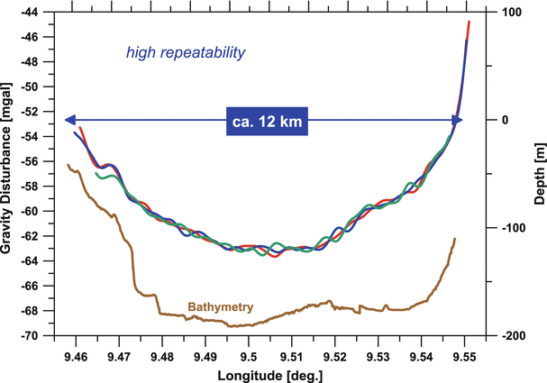
Gravity disturbances measured three times along the same profile (see Fig. 2) on lake Constance
-
June 2013: Oderhaff (Szczecin Lagoon) and an Ostsee (Baltic Sea) area adjacent to Poland – cooperation with BKG.


The 2 days mission on Lake Müritz was the first performance test of the new gravimeter. One profile (see Fig. 2) was measured seven times. Figure 3 shows the achieved high repeatability of the gravity measurements (within 1 mgal) at a resolution of ca. 400 m. The main purpose of the other two campaigns (accomplished in cooperation with BKG) was refining the existing gravity data and improving the geoid modeling in these border regions between Germany and neighboring countries (Schäfer et al. 2013). Very good performance of the gravimeter was confirmed again (Fig. 4). High quality results obtained with this type of instrument in shipborne gravimetry are already known from the literature (Zheleznyak 2010). Nevertheless, since gravimeters are no mass products, it is advisable to test the performance of every individual specimen.
3 Airborne Gravimetry in the Frame of GEOHALO Mission
In the first half of June 2012 our first airborne gravity campaign using Chekan-AM took place as part of the multidisciplinary geoscientific airborne mission GEOHALO. The project covered the Italian Peninsula and surroundings and was accomplished by an international group of scientific and exploration institutions, see Scheinert et al. (2013) and Fig. 5. The mission was flown on the German High Altitude and LOng Range Research Aircraft (HALO), which is a modification of the business jet G550 (Gulfstream Aerospace Corporation). Hence, a jet aircraft was used flying at a higher altitude and with higher speed than it is usual for exploration purposes. In contrast to geophysical exploration (maximum resolution at the lowest flight speed and altitude possible) the leading idea was to demonstrate the possibility to cover a wide region in a realistic time span achieving the resolution needed to refine a global satellite-only gravity model in areas with sparse terrestrial data or to close the so-called “polar gap” (due to the satellites’ inclinations) of dedicated satellite gravity field missions.

Flight tracks of the 4 day mission, the results for two tracks (black dotted lines) are presented as example (Fig. 8)
The parameters of the mission were: total length of all profiles of about 16,150 km, effective measurement time of circa 33 h, mostly at an altitude of approximately 3,500 m, and an average speed of 425 km/h.
3.1 Data Processing Along Individual Profiles
The principles of airborne gravimetry can be found for instance in Forsberg and Olesen (2010). We applied the processing scheme presented by Krasnov et al. (2011b).
The recovery of gravimeter readings along the trajectory of the aircraft is based on the mathematical model and calibration constants provided by the manufacturer of the instrument. In order to calculate the gravity values (at flight altitude) the Eötvös correction (Jekeli 2001, eq. 10.95, p. 334) and the vertical component of the kinematic acceleration have to be subtracted. The last mentioned component is usually computed by numerical double differentiation of the position from GNSS. Due to the higher speed of the HALO aircraft, this procedure did not give satisfactory results and the inclusion of Doppler observations into the GNSS processing seems necessary.
Since all mentioned acceleration components contain high-frequency noise they have to be low-pass filtered, applying the same filter characteristics. A 100 s low-pass filter, used in data processing, corresponds at the aircraft speed of about 120 m/s to a spatial resolution of about 12 km (half wave length).
The gravimeter recordings taken before and after the flights always at approximately the same position were used to eliminate the drift of the gravimeter. After correcting the drift, the relative gravity values along the trajectories can be transformed into absolute gravity values using an appropriate gravity datum. For this, a local relative gravity survey was conducted during the time of the GEOHALO mission to link a local marker at the apron with gravity reference points in the vicinity of the airfield.
The investigations of several aspects, including the influence of the chosen way of GNSS processing, different low-pass filters, etc., are still going on and the outcome presented here has to be regarded as a first preliminary result.
3.2 Possibilities to Check the Collected Data
First, we eliminated approximately (only) 5% of the recordings which are definitively not usable (recordings immediately after the change of track, some short periods of too strong turbulences, and similar). The waste in airborne gravimetry is usually larger. We retained for the moment all data (Fig. 6) which might be usable at the end or should be analyzed for the reasons of mismatches.

Gravity disturbances on the ellipsoid of the satellite-only model EIGEN-6S and the locations of usable data of the GEOHALO mission
After this, 19 cross-over points are obtained; 4 of them are obviously outliers, and will be analyzed in more details in future. The remaining 15 are obviously too few for any serious statistics (holds also for 19), and especially for any cross-over adjustment. Nevertheless, let us mention that the mean cross-over difference is 0.5 mgal, the mean of the absolute values of differences 2.9 mgal, and their RMS-difference 3.4 mgal. As explained, these values should not be over-interpreted.
Because there are only so few cross-over points, a detailed error analysis can only be done by comparisons with accurate ground data which is planed for future work in cooperation with Italian colleagues.
However, if airborne gravimetry is used not only to measure the gravity field along some special profiles but over a given region, as it was in our case, it has to be taken into account that the spatial resolutions along-track and cross-track are two different issues.
For this mission the along track resolution is about 12 km (see Sect. 3.1). The cross-track resolution is directly given by the track distance. For the GEOHALO mission the track distance of 40 km was a good balance between the different objectives of the participating multidisciplinary teams and the budget.
In areas where no or only sparse (or bad) terrestrial data are available the only gravity field information comes from the global satellite-only gravity field models. These models are represented mathematically in terms of spherical harmonics and recent models have maximum degrees and orders from N max = 230 to N max = 260 which corresponds to a best possible spatial resolution, i.e. smallest representable bumps and dales, of ca. 80–100 km (see e.g. Barthelmes 2013, table 1). Figure 6 shows the gravity disturbances of the model EIGEN-6S (Förste et al. 2013) (N max = 240, data from LAGEOS, GRACE AND GOCE) for the Italian region. Additionally, the positions of the usable data of the mission are drawn.
The most recent global gravity field model which, additionally to satellite data, contains data from altimetry over the oceans, and terrestrial gravity measurements over the continents, is the model EIGEN-6C2 (Förste et al. 2013). The maximum degree and order of this spherical harmonic model is N max = 1949 which corresponds to a best possible resolution of ca. 10–12 km. However, this resolution is only realized in regions where good and dense data are integrated into the model. Fortunately, this is the case for the Italian region and we can use this model for a first rough evaluation of the airborne gravity data. Figure 7 shows the gravity disturbances of this model for the area of interest.

Gravity disturbances on the ellipsoid of the model EIGEN-6C2
3.3 Comparison with the Global Model EIGEN-6C2
As a first step, the measurements along the tracks can be directly compared to the values computed from the model EIGEN-6C2 at the same points. Figure 8 shows these comparisons for the two tracks marked in Fig. 5. The normal gravity at the points has been subtracted; thus, the values are gravity disturbances at flight height. The curves show the expected resolution of about 10–12 km and the good match between the model and the measurements. The difference between our measurements and the global model EIGEN-6C2, marked with a red ellipse in Fig. 8, might be a result of the well-known oscillating behavior of a truncated spherical harmonic series at locations where structures with sharp edges should be approximated. Analogous comparisons with the model EIGEN-6C2 have been done for all tracks and show similar concordance. Although the final interpretation of the differences between the model and the measurements should be done in more detail after the final data processing, the quick visual comparison with EIGEN-6C2 gives an impression of the reliability of the airborne gravity measurements.

Gravity disturbances measured along the two profiles displayed in Fig. 5 (eastern track: top, western track: bottom) and computed from the model EIGEN-6C2, both at flight altitude. Topography and bathymetry are also shown
To use airborne gravity measurements for geodetic purposes in particular, if we want to compute geoid undulations from these data, and the measurements should be compared or combined with ground data and satellite derived models, the best way seems to be to compute a harmonic function approximation which fits the data. The limit for the resolution of such a function is the 40 km track distance because we don’t want to have a non-isotropic spatial resolution. This corresponds to a spherical harmonic representation with maximum degree and order of approximately N max = 600. Figure 9 shows the gravity disturbances of the model EIGEN-6C2 truncated at degree \(N = N_{\mathit{max}} = 600\), which gives an impression what can be expected by modeling the gravity measurements of the GEOHALO mission. This means that airborne gravity campaigns such as the GEOHALO-mission should be able to improve the globally available resolution of 80–100 km of the satellite-only models (Fig. 6) to a resolution of about 40 km shown in Fig. 9.

Gravity disturbances on the ellipsoid of the model EIGEN-6C2 up to N max = 600. This is the resolution expected due to the 40 km track distance
To demonstrate this in a first simple test we computed a point mass model with fixed positions and a fixed uniform depth by least squares fitting the masses to the measured gravity values. For this, the masses were distributed along the tracks at a distance and depth corresponding to the expected resolution limited by the 40 km track spacing. Thus, 40 km has been chosen for the depth and for the mean distance of the masses along the tracks, but no masses were placed under data gaps. From the gravity measurements at flight height the normal gravity has been subtracted and these data has been used to compute the magnitudes of the 236 masses by a least squares fit. The method of approximating the gravity field by point masses has been described in the past in many publications. Overviews are given e.g. by Barthelmes (1986, 1989), Barthelmes and Dietrich (1991), Claessens et al. (2001), and Klees et al. (2008). The resulting gravity disturbances of this point mass model on the ellipsoid are shown together with the positions of the masses in Fig. 10. The Figs. 9 and 10 show very good agreement in all details, which confirms the quality of the airborne measurements.

Gravity disturbances on the ellipsoid of the point mass model (236 masses) computed alone from the airborne gravity values at flight height
For geoid computations from data of such a mission a satellite-only model should be subtracted prior to the fit of the harmonic function (and has to be added afterwards) to minimize the (long-wavelength) influence of the areas without measurements outside the region. If high resolution topography information is available, it should be used too. In areas where good ground data are available (like in our case) such airborne missions with long tracks can be used to homogenize the ground data. These topics as well as a detailed error analysis of the measurements are tasks for the future.
4 Conclusions and Outlook
Shipborne gravity campaigns confirmed the high repeatability of the measurements performed by the gravimeter CHEKAN-AM.
The GEOHALO experiment confirmed reasonable agreement with a high resolution global gravity field model (which is based on good terrestrial data in this region). Furthermore, this experiment resulted in resolution and accuracy suitable for establishing links between satellite and terrestrial gravity measurements. In particular, it can be concluded that the equipment is very well suited for improving global combined (satellite-terrestrial) gravity field models in regions with sparse terrestrial data coverage.
References
Barthelmes F (1986) Untersuchungen zur Approximation des äußeren Gravitationsfeldes der Erde durch Punktmassen mit optimierten Positionen. Veröffentlichungen des Zentralinstituts für Physik der Erde 92, Zentralinstitut für Physik der Erde, Potsdam. http://www.gfz-potsdam.de/bib/pub/digi/barthelmes_diss1986.pdf
Barthelmes F (1989) Local gravity field approximation by point masses with optimized positions. In: 6th international symposium “geodesy and physics of the earth”. Veröffentlichungen des Zentralinstituts für Physik der Erde, vol 102, Part 2, pp 157–167. ftp://ftp.gfz-potsdam.de/pub/home/sf/bar/publications/pm-local_89.pdf
Barthelmes F (2013) Definition of functionals of the geopotential and their calculation from spherical harmonic models: theory and formulas used by the calculation service of the international centre for global Earth models (ICGEM); http://icgem.gfz-potsdam.de/ICGEM/. Scientific Technical report STR09/02, Revised edition, January 2013, GeoForschungZentrum Potsdam. doi:10.2312/GFZ.b103-0902-26. http://gfzpublic.gfz-potsdam.de/pubman/item/escidoc:104132
Barthelmes F, Dietrich R (1991) Use of point masses on optimized positions for the approximation of the gravity field. In: Rapp R, Sansò F (eds) Determination of the geoid: present and future. International association of geodesy symposia. Springer, New York, pp 484–493
Claessens S, Featherstone W, Barthelmes F (2001) Experiences with point-mass modelling in the Perth region, Western Australia. Geo Res Aust 75:53–86
Forsberg R, Olesen AV (2010) Airborne gravity field determination. In: Xu G (ed) Sciences of geodesy - I. Springer, Berlin, pp 83–104. doi:10.1007/978-3-642-11741-1_3. http://dx.doi.org/10.1007/978-3-642-11741-1_3
Förste C, Bruinsma S, Flechtner F, Marty JC, Dahle C, Abrikosov O, Lemoine JM, Neumayer KH, Barthelmes F, Biancale R, König R (2013) A new combined global gravity field model including GOCE data up to degree and order 1949 of GFZ Potsdam and GRGS Toulouse. Paper presented at the general assembly European geosciences union, Vienna, 3–7 December 2013
Jekeli C (2001) Inertial navigation systems with geodetic applications. De Gruyter, Berlin [u.a.]. http://books.google.de/books?id=9OLlnQEACAAJ
Klees R, Tenzer R, Prutkin I, Wittwer TF (2008) A data-driven approach to local gravity field modelling using spherical radial basis functions. J Geod 82(1):457–471
Krasnov A, Nesenyuk L, Peshekhonov V, Sokolov A, Elinson L (2011a) Integrated marine gravimetric system. Development and operation results. Gyroscopy Navig 2(2):75–81. doi:10.1134/S2075108711020052. http://dx.doi.org/10.1134/S2075108711020052
Krasnov A, Sokolov A, Usov S (2011b) Modern equipment and methods for gravity investigation in hard-to-reach regions. Gyroscopy Navig 2(3):178–183. doi:10.1134/S2075108711030072. http://dx.doi.org/10.1134/S2075108711030072
Schäfer U, Liebsch G, Rülke A, Schirmer U, Barthelmes F, Petrovic S, Pflug H (2013) Recent ship-borne gravity campaigns in Germany—motivation, design and first results. Paper presented at the IAG Scientific Assembly, Potsdam, 1–6 September 2013
Scheinert M (2010) Progress in the regional determination of the Antarctic geoid. Poster presented at the SCAR open science conference, Buenos Aires, 3–6 August 2010
Scheinert M, Petrovic S, Heyde I, Barthelmes F, The GEOHALO Group (2013) The geodetic-geophysical flight mission GEOHALO: results of airborne gravimetry and further geodetic products. Paper presented at the IAG scientific assembly, Potsdam, 1–6 September 2013
Stelkens-Kobsch T (2005) The airborne gravimeter Chekan-A at the institute of flight guidance (IFF). In: Jekeli C, Bastos L, Fernandes J (eds) Gravity, geoid and space missions. International association of geodesy symposia, vol 129. Springer, Berlin, pp 113–118. doi:10.1007/3-540-26932-0_20. http://dx.doi.org/10.1007/3-540-26932-0_20
Zheleznyak L (2010) The accuracy of measurements by the CHEKAN-AM gravity system at sea. Izv Phys Solid Earth 46(11):1000–1003. doi:10.1134/S106935131011008X. http://dx.doi.org/10.1134/S106935131011008X
Acknowledgements
The financial contribution of the German Research Foundation (DFG) in the frame of SPP 1294 (“High Altitude and LOng Range Research Aircraft”) is gratefully acknowledged. The realization of the described mission was made possible by the efforts of all members of the GEOHALO team, especially of its coordinator Mirko Scheinert. We are also grateful to the Federal Agency for Cartography and Geodesy (BKG) for pleasant cooperation in two shipborne campaigns and especially for the big engagement in solving all logistic and organizational problems. Last but not least, we thank Anton Krasnov from the manufacturer of our gravimeter Chekan-AM, Concern CSRI Elektropribor (Saint Petersburg, Russia) for his helpfulness in solving questions connected with the functioning of the instrument.
Author information
Authors and Affiliations
Editor information
Editors and Affiliations
Rights and permissions
Copyright information
© 2015 Springer International Publishing Switzerland
About this paper
Cite this paper
Petrovic, S., Barthelmes, F., Pflug, H. (2015). Airborne and Shipborne Gravimetry at GFZ with Emphasis on the GEOHALO Project. In: Rizos, C., Willis, P. (eds) IAG 150 Years. International Association of Geodesy Symposia, vol 143. Springer, Cham. https://doi.org/10.1007/1345_2015_17
Download citation
DOI: https://doi.org/10.1007/1345_2015_17
Published:
Publisher Name: Springer, Cham
Print ISBN: 978-3-319-24603-1
Online ISBN: 978-3-319-30895-1
eBook Packages: Earth and Environmental ScienceEarth and Environmental Science (R0)